CS224N Lecture 1 — Introduction and Word Vectors
Course: Stanford CS224N / Ling284, Natural Language Processing with Deep Learning
Lecture: Lecture 1 — Introduction and the History of NLP (guest lecture by Prof. Christopher Manning, the creator of CS224N)
Video: Stanford CS224N: NLP with Deep Learning | Lecture 1 — video ID DzpHeXVSC5I, 4817 s (≈ 80 min)
Course homepage: cs224n.stanford.edu (a.k.a. stanford.edu/class/cs224n)
Course materials used for this book: the two deck PDFs shipped with the recording — cs224n-2026-lecture01-history.pdf (the history deck) and cs224n-2026-lecture01-intro.pdf (the course-introduction and word-vectors deck). Slide titles are quoted below as short references; no slides are reproduced wholesale.
导览
This is a 3–5 minute map of the lecture. It says what questions are on the table, where the road gets steep, and in what order the answers arrive. It deliberately does not summarize the answers.
1. The questions the lecturer actually asks, in his own order.
- What is this course for? He answers with three learning goals (deep-learning foundations for NLP, a big-picture understanding of human language, and the ability to actually build systems), then spends ten minutes on logistics before touching any content.
- Why is language the one thing that really separates us from our nearest relatives? And a follow-up he insists on: is language only for communication, or is it also a tool for thinking?
- What changed in the last decade? Machine translation, then GPT-2, then ChatGPT/GPT-4 — the question is what these systems can and cannot do, in his own examples.
- What does "meaning" mean? Where do you keep the meaning of a word inside a computer? He works through the dictionary/denotational answer, then WordNet, and shows why each one fails.
- What if a word's meaning were simply its context? This is the pivot of the whole lecture.
- What exactly is the word2vec algorithm, what is its objective function, and how do you compute the gradient that trains it? This last question is the technical core, and it is where the lecture runs out of time.
2. Where it gets hard. Three places.
- The conceptual switch from "meaning = the thing a symbol stands for" to "meaning = a vector learned from co-occurrence". Nothing in a dictionary can be gradient-descended; something in a corpus can.
- The softmax step: why exponentiate, why normalize, and why the resulting quantity is a probability distribution over the entire vocabulary rather than a comparison between two words.
- The back half of the derivation: a quotient inside a logarithm, then the chain rule applied twice, then a component-by-component derivative of a dot product. Manning warns the audience himself that this ten-minute stretch will be trivial for some and impenetrable for others, and tells the second group that this is exactly why he is doing it slowly.
3. Questions you may be bringing in. Kept in two groups, as they should be.
① Questions raised by the lecturer, or by students in the room:
- How many dimensions should a word vector have, and how do you choose?
- Are the entries of a word vector bounded?
- Does only distance in the space carry meaning, or also direction?
- A word like star has several senses — can one vector handle that?
- Why does the model need two vectors per word?
- (From the lecturer himself) why do we minimize instead of maximize?
② Questions the editor predicts you will have (editor's guesses, not the lecturer's):
- What exactly is a "corpus", and why is the plural not "corpys"?
- In one line, what is the difference between a one-hot vector and an embedding?
- Is the algorithm taught here skip-gram or CBOW? The lecture never says, and the derivation shown corresponds to one of them.
- Where do the BLEU numbers in the machine-translation chart come from?
- If WordNet is so flawed, why is it still around?
4. The route. Course logistics (about ten minutes) → human language and what meaning is → the shape of NLP history, in four eras → the deep-learning breakthroughs, told through machine translation, GPT-2, ChatGPT/GPT-4 and image generation → "meaning" as denotation, and WordNet's failure → word vectors and distributional semantics → word2vec, softmax, and the gradient derivation, which is cut off by the end of class.
1. Course Overview: What CS224N Sets Out to Teach
(reference time: 00:00:05)
Manning opens with an observation about the course itself: it was taught just the previous quarter, and here is another enormous cohort taking it again. His guess at what that says is, in his words, roughly "ChatGPT" — a wry explanation for why a specialized NLP class is now full.
The lecture plan he announces is: a few minutes on the course, a few remarks on human language and word meaning, and then the main technical content — the word2vec algorithm, which he describes as a little over a decade old (introduced in 2013), wildly successful, and a simple way of learning vector representations of words. He frames it as a deliberately easy "baby system" for the kind of neural representations the rest of the course is about: it is the first model whose objective function, gradients and optimization the class can fully work through by hand.
(reference time: 00:02:24 — course logistics)
Logistics, briefly and only as far as it explains the teaching philosophy:
- Instructor and course staff: the head TA is absent that day for health reasons, the course manager is in the room, and the TAs are on the website. The main channel for information and questions is the course website, which links to Ed as the discussion board — Manning explicitly asks students to use Ed rather than email him.
- The first assignment is already live and due the following Tuesday, before class: "slightly less than seven days". Office hours start the next day; the first Friday tutorial is on Python and NumPy, offered precisely because the class wants to be accessible to people who have not done that yet.
- Editor's note: the posted deck also lists a PyTorch tutorial on the second Friday. The whole course is built on Python plus PyTorch, so these two tutorials are not optional garnish for beginners.
1.1 The three learning goals
(reference time: 00:04:30)
Manning states three goals, and says the end-of-quarter evaluation will ask students whether the class met them.
- The foundations and current methods for applying deep learning to NLP. The course builds bottom-up: word vectors, feed-forward networks, recurrent networks, attention, then Transformers and encoder–decoder models. He notes mid-sentence that he probably should have written large language models into the slide as well, and adds pre-training and post-training, adaptation, interpretability and agents to the list of 2024-era topics.
- A sense of human language and why it is hard for computers. He makes a pointed remark here: only a few students are Linguistics or Symbolic Systems majors — "yay to the Symbolic Systems majors" — and for most of the rest of the class, this will be the only place where they see how language works and why understanding it is difficult, even though humans find it easy.
- Building real systems. The stated goal is that a student should leave thinking: "in my first job, at a startup, big tech, or a nonprofit, if they need a text classification system or information extraction to pull facts out of documents, I can build that — because I did CS224N." He is explicit that this is not meant to be a theory-only class.
1.2 Grading, collaboration, and the AI-tools policy
(reference time: 00:07:05)
The grade splits roughly in half between coursework and a project:
- Four assignments, each about a week and a half long. The first is worth 6%, the other three 14% each, for 48% total.
- A final project (49%), either the default project (with a lot of scaffolding) or a custom project that the staff approves; teams of 1–3 students may use any language and packages. The project is broken into proposal (8%), milestone (6%), poster or web summary (3%) and report (32%).
- Participation (3%), plus a late-day policy of six free late days and 1% of the course grade per day after that.
Two policies get real airtime:
- Collaboration. Students may talk to friends, but must write and submit their own assignment solutions, and must document collaboration. For the final project, group work is expected and allowed.
- AI tools. The framing is careful and worth quoting in substance: "in this class we love large language models, but we don't want you to do your assignments by saying 'hey ChatGPT, could you answer question three for me?' That is not the way to learn things." Using AI as a coding assistant is fine; outsourcing the reasoning behind an assignment answer is a violation.
1.3 What the assignments actually ask you to do
(reference time: 00:08:40)
- HW1 is an easy on-ramp, delivered as a Jupyter notebook.
- HW2 is where the class wants mathematics and an understanding of how neural networks work, and it is where PyTorch is introduced; students build a small network for dependency parsing. Manning is candid: "for some people, assignment two is the scariest assignment in the whole class." He also justifies the math with a line about institutional identity — at a university that is "this fine liberal arts and engineering institution, not a coding boot camp", the goal is deep understanding, not just working code.
- HW3 and HW4 move to larger projects using PyTorch on GPUs, with Google Cloud as the compute provider, covering machine translation and information extraction with Transformers.
- The final project is either the default option (implement a GPT, then fine-tune and adapt it for downstream tasks, with substantial scaffolding) or a self-proposed project. A student asks how mentors are assigned; Manning's answer is that students may find their own mentor if they have a specific interest and someone agrees, otherwise the TA in charge of final projects distributes students across course staff as evenly as possible.
2. Human Language and Word Meaning: Why Language Is So Special
(reference time: 00:11:20)
Manning introduces himself as a linguist and gives what he calls his biased take. Compare humans with our nearest neighbours — chimpanzees and bonobos — and the differences are surprisingly thin. They use tools, they plan how to solve problems, and their memory is not merely comparable: chimpanzees have better short-term memory than humans. On most axes it is hard to demonstrate an intelligence gap, "except for the fact that we have language".
Then the observation that gives language its weight: there are creatures stronger, faster, more venomous than us, with every conceivable physical advantage, and human beings took over the planet anyway. How? Language — because it allowed communication, and communication allowed human ascendancy.
But Manning argues that communication is not the only role of language:
- Some thought clearly requires no language — imagining a scene, mentally moving furniture around, feeling scared or excited.
- Most higher-level cognition, though, runs in language. His example is deliberately ordinary: you notice your friend seemed upset about what you said last night, and you think through how to fix that, plan what to say, run the conversation in your head. Language gives us a scaffolding for more detailed thought and planning.
(reference time: 00:14:30)
The second half of the argument is about writing:
- Nobody knows exactly how old human languages are; most estimates are a few hundred thousand years, which is not long on an evolutionary timescale.
- Writing, by contrast, is known and recent: about 5,000 years old. And writing turned out to be an enormous cognitive tool, because it allowed knowledge to be shared across time and space, not only with the people standing within fifty feet of you. Manning's framing is that writing alone was enough to take humanity from Bronze-Age metalworking to the mobile phones we carry — in a very short amount of time. "Language is pretty cool."
(reference time: 00:15:45)
He then pushes back on fixating solely on the knowledge function of language. Language is also a social tool, a very flexible system used with imprecision, nuance and emotion, and one that can set up new ways of thinking simply by giving them words. Two consequences matter for the rest of the course:
- Languages are not static and were not "delivered down on tablets by God". They are constructed and changed by their users — and most of the innovation happens among young people, in early teens through the twenties.
- He closes with a quotation from the retired Stanford psychologist Herb Clark: "The common misconception is that language use has primarily to do with words and what they mean. It doesn't; it has primarily to do with people and what they mean."
Editor's note: why this matters technically, not just philosophically. Clark's point is the reason a purely lexical, dictionary-style semantics will fail later in this lecture: words are tools people use with intent, and their meaning shifts with use. The statistical approach that replaces the dictionary does not solve this, but it does take the usage — the company a word keeps — as its raw material.
3. The Shape of NLP History: Four Paradigm Shifts
(reference time: 00:17:30)
Manning gestures at the history here — "we'll say a bit more about the history later on" — and the course's history deck supplies the framework that the whole lecture, and arguably the whole course, is organised around: four eras of NLP.
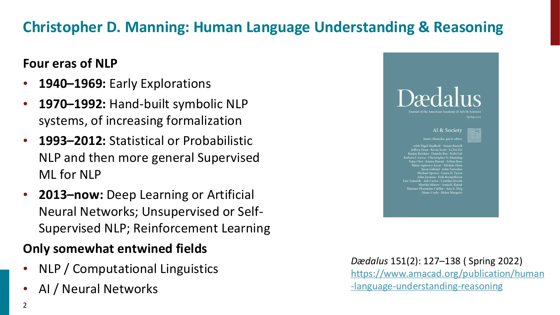
📷 Christopher Manning's four-era map of NLP, used to frame the whole lecture and the course
回到原视频 (00:17:40)
- 1940–1969 — Early explorations. Machine translation as the origin of computational linguistics, the Dartmouth workshop, cybernetics and the first mathematical neuron, information retrieval, the first benchmarks.
- 1970–1992 — Hand-built symbolic NLP systems, of increasing formalization. Formal and unification-based grammars, knowledge representation and inference, natural-language understanding demos, and then the symbolic wall and the "AI winter".
- 1993–2012 — Statistical or probabilistic NLP, then more general supervised ML for NLP. The influx of ideas from electrical engineering and speech recognition, machine-readable corpora, annotated training data, empirical evaluation, and deliberately lowered ambitions.
- 2013–now — Deep learning / artificial neural networks, unsupervised or self-supervised NLP, plus reinforcement learning. Neural word vectors, encoder–decoder sequence models, Transformers, and large language models.
The framework has two structural claims that the lecture leans on repeatedly:
- NLP/computational linguistics and AI/neural networks are only somewhat entwined fields. Tracing them as two strands, rather than one, is what makes the alternating fortunes of symbolic and statistical methods intelligible.
- The stated key learning for the day: understand the paradigm shifts in NLP and how our assumptions about language shape what is possible in each era. This is the sentence that ties the history section to the technical sections: each era's definition of "language" bounds what its systems can do.
graph LR
    A["1940–1969<br/>Early explorations<br/>MT, cybernetics, IR, benchmarks"] --> B["1970–1992<br/>Hand-built symbolic NLP<br/>increasing formalization"]
    B --> C["1993–2012<br/>Statistical / probabilistic NLP<br/>then supervised ML"]
    C --> D["2013–now<br/>Deep learning, self-supervision<br/>+ reinforcement learning"]
Editor's extension — where the four-era framing comes from. The four eras, and the phrase "only somewhat entwined fields", come from Manning's own essay Human Language Understanding & Reasoning (Dædalus 151(2), 2022), which is cited on the slide and is the written companion to this lecture. Two useful details that the ten-minute spoken version compresses: the era boundaries are fuzzy and overlapping — the statistical revolution begins in speech recognition in the 1970s, decades before it takes over NLP — and the fourth era is not purely a story about neural networks, but about the combination of neural networks, self-supervised objectives, and vastly more data and compute.
Editor's note on this recording. In this particular video, the long history segment (roughly an hour of material in the course's own plan) is not delivered in full; the transcript jumps from the four-era overview to the modern deep-learning results. The history deck that is shipped with the recording is the source for the era summary above. See Known Uncertainties at the end of this book.
4. The First Deep Learning Breakthrough: Neural Machine Translation
(reference time: 00:18:10)
Manning asks the audience to appreciate how young this field of progress is. Work on doing things with human language started in the 1950s, so it had been going for about sixty years, and the ability to understand and produce language had "always been kind of questionable" — until neural networks produced enormous strides in roughly the last decade.
The first big breakthrough came in machine translation:
- It started around 2014.
- By 2016 it was deployed live in services like Google Translate.
- It was good enough that commercial deployment was very rapid — Manning's point is that this was not a research curiosity that took a decade to reach users.
The architecture behind those first systems was the encoder–decoder network, and the lecture's example is deliberately small: read "I am a student", produce "Je suis étudiant". The encoder reads the source sentence word by word and builds up a representation of its meaning; the decoder generates the translation word by word, fed the previous word it produced.
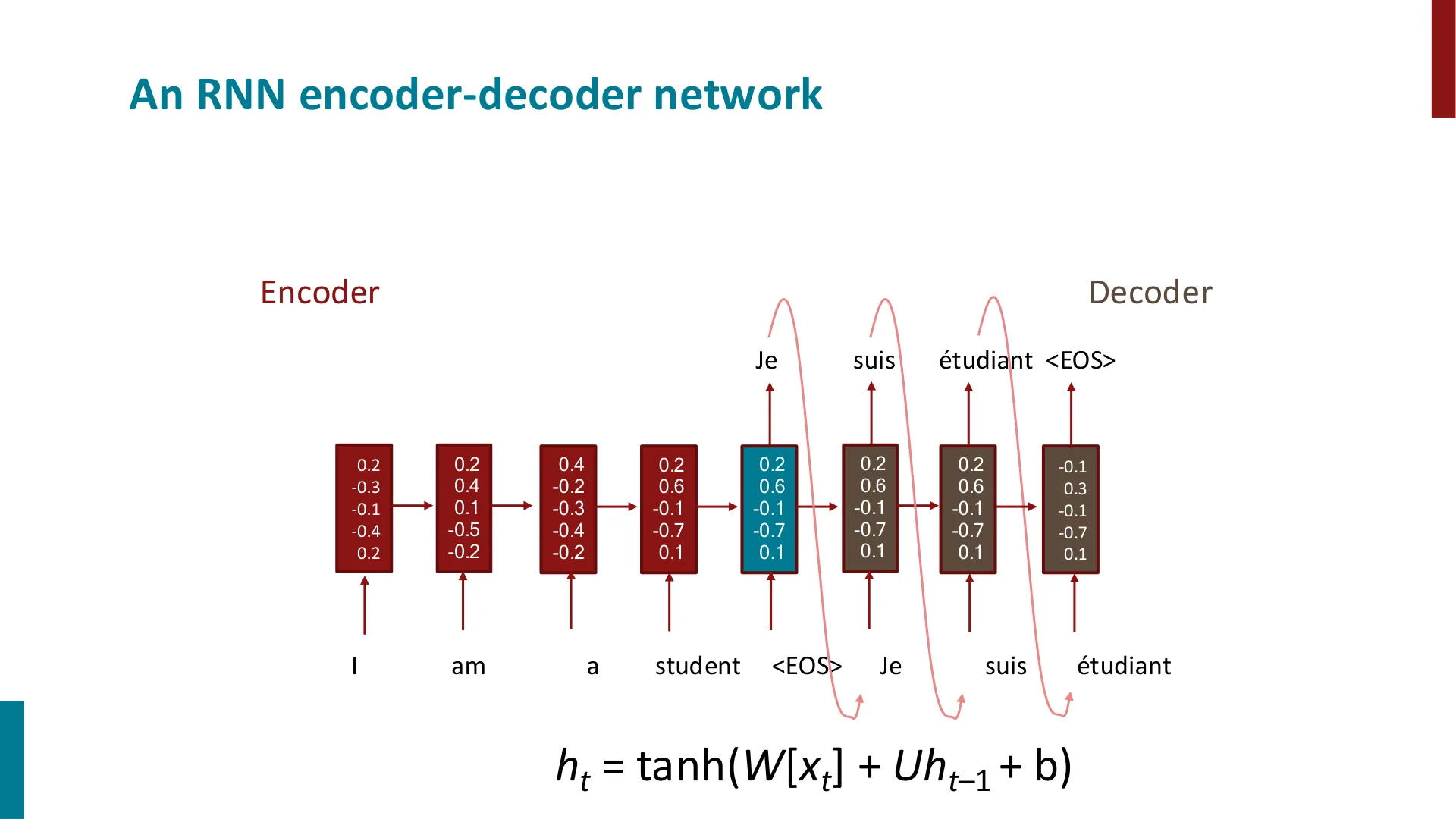
📷 The RNN encoder–decoder architecture for machine translation: reading the source sentence, compressing it into a vector, generating the translation
回到原视频 (00:18:25)
The recurrent cell in the deck is the standard one:
$$h_t = \tanh\!\left(W[x_t] + U h_{t-1} + b\right)$$
Quality is measured with BLEU (a score comparing the system output against reference translations), and the numbers move fast: on English–German news translation, phrase-based and syntax-based statistical MT give way to neural MT with a large jump in just a few years.
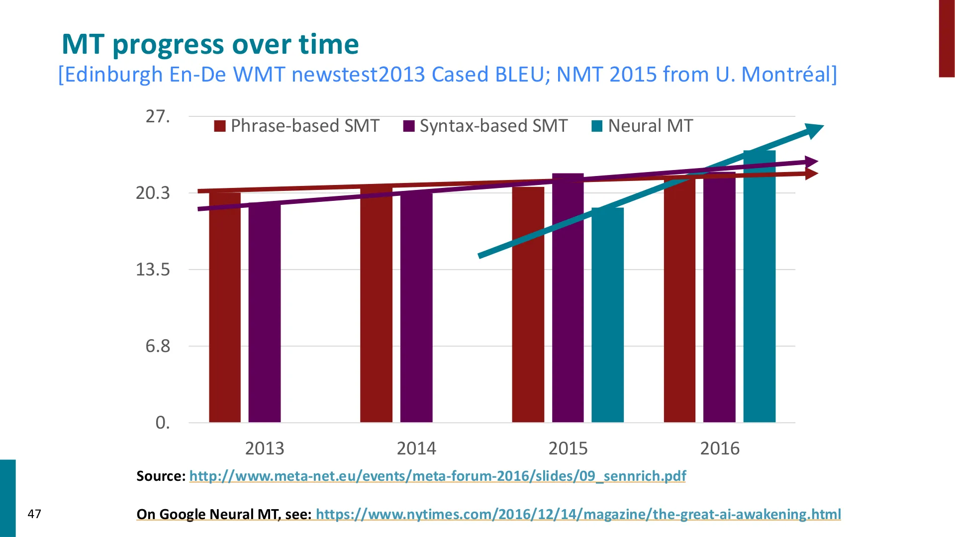
📷 BLEU on English–German newstest2013 rising sharply as neural MT replaces phrase-based and syntax-based statistical MT
回到原视频 (00:18:52)
(reference time: 00:19:05)
What this means to a student, in Manning's telling, is a different world from a few generations back. Then, unless you had learned another language, you had essentially no way to communicate with people who spoke it. Now we are close to something like the Babel Fish from The Hitchhiker's Guide to the Galaxy — except, as he puts it, "it's not a Babel Fish, it's a cell phone": you can put it between two people and get simultaneous translation. It is not perfect, and research continues, but the practical consequence is that you can pick up information from anywhere. His example is a Swahili news snippet from Kenya, which he can paste into a translation service and learn from: Malawi lost two ministers to COVID infections.
graph LR
    S["Source sentence<br/>I am a student [EOS]"] --> E["Encoder: builds up sentence meaning<br/>h_t = tanh(W[x_t] + U h_(t-1) + b)"]
    E --> V["Bottleneck: one vector for the sentence"]
    V --> D["Decoder: generates one word at a time"]
    D --> O["Translation<br/>Je suis étudiant [EOS]"]
Editor's extension — what BLEU actually measures. BLEU counts how many n-grams of the system output also appear in one or more human reference translations (usually up to 4-grams), takes a weighted geometric mean, and applies a brevity penalty so that a system cannot win by emitting very short outputs. It is cheap, automatic, and correlates only moderately with human judgement — which is why the shape of the curve in the slide (a rapid, large improvement) is the meaningful part, not the absolute numbers.
Editor's extension — why the encoder–decoder design was a breakthrough and also a bottleneck. Compressing an entire source sentence into a single fixed-length vector is the design flaw that the next lecture's attention mechanism removes: the decoder gets one vector to condition on, no matter how long or complex the source sentence is. The word "bottleneck" on the slide is precisely this.
5. The Rise of Large Language Models and Generative AI
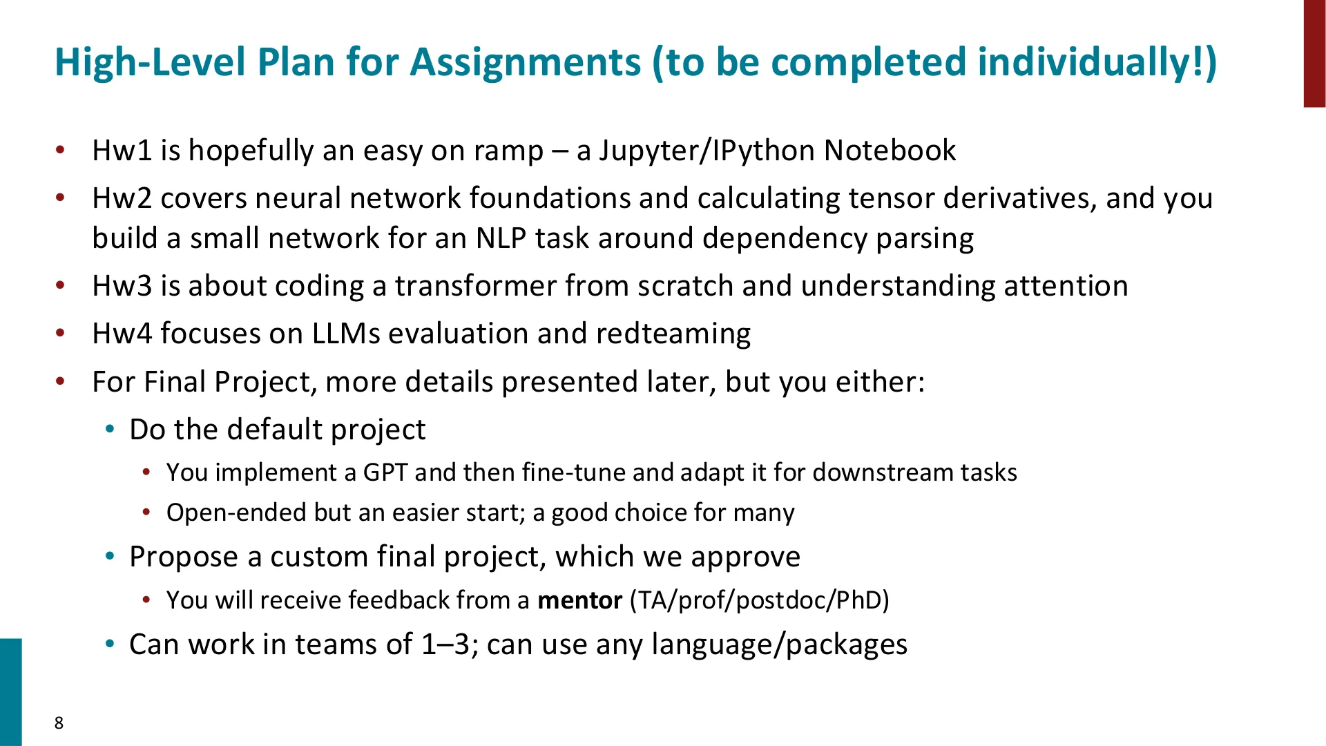
🖼️ Manning walks through what each assignment covers (HW1 notebook, HW2 neural network foundations and dependency parsing, HW3 a transformer from scratch, HW4 LLM evaluation) and both final-project options; this page is the clean summary of that walkthrough.
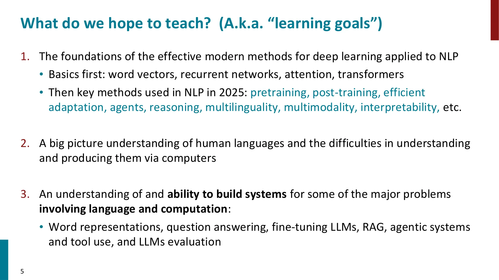
🖼️ This page states the three learning goals Manning spends the first part of the lecture explaining (foundations of deep learning for NLP, a big-picture understanding of human language, and the ability to build systems), so it serves as the roadmap for the opening section.
(reference time: 00:20:10)
Before turning to language models, Manning notes a second way neural networks had already changed everyday products: search stopped being keyword matching and became an answer engine. A few years ago, you typed something and got back pages that might contain the answer, matched against an index. Now you can type an actual question — his example is "when did Kendrick Lamar's first album come out?" — and the system finds relevant documents, reads them, and returns an answer.
Architecturally, that is a pipeline of several networks, and the lecture names three stages.
graph LR
    Q["User question"] --> R["Retrieval network<br/>finds passages similar to the query"]
    R --> K["Reranking network<br/>reorders the candidates"]
    K --> RD["Reading network<br/>synthesises an answer from the passages"]
    RD --> A["A returned answer, not a list of links"]
(reference time: 00:21:35 — GPT-2)
Then he gets to what he calls the moment things got more advanced again. Around 2019, people in NLP started to see the power of large language models, and those of us in the field were genuinely excited about GPT-2. His caveat is lovely and honest: GPT-2 "didn't make much of an impact on the nightly news", but in NLP it mattered because, for the first time, here was a large language model that could generate fluent text. Until then, NLP systems had done a decent job of extracting facts from text, but nobody could generate fluent text at all.
The core mechanism is as simple as it sounds: given some preceding text, predict the next word; generate the text one word at a time. His demonstration is an invented news story. He gives GPT-2 the opening line about a train carriage containing controlled nuclear materials being stolen in Cincinnati. GPT-2 continues with a plausible news report: the incident occurred on the downtown train line, the US Department of Energy is working with the Federal Railroad Administration to find the thief.
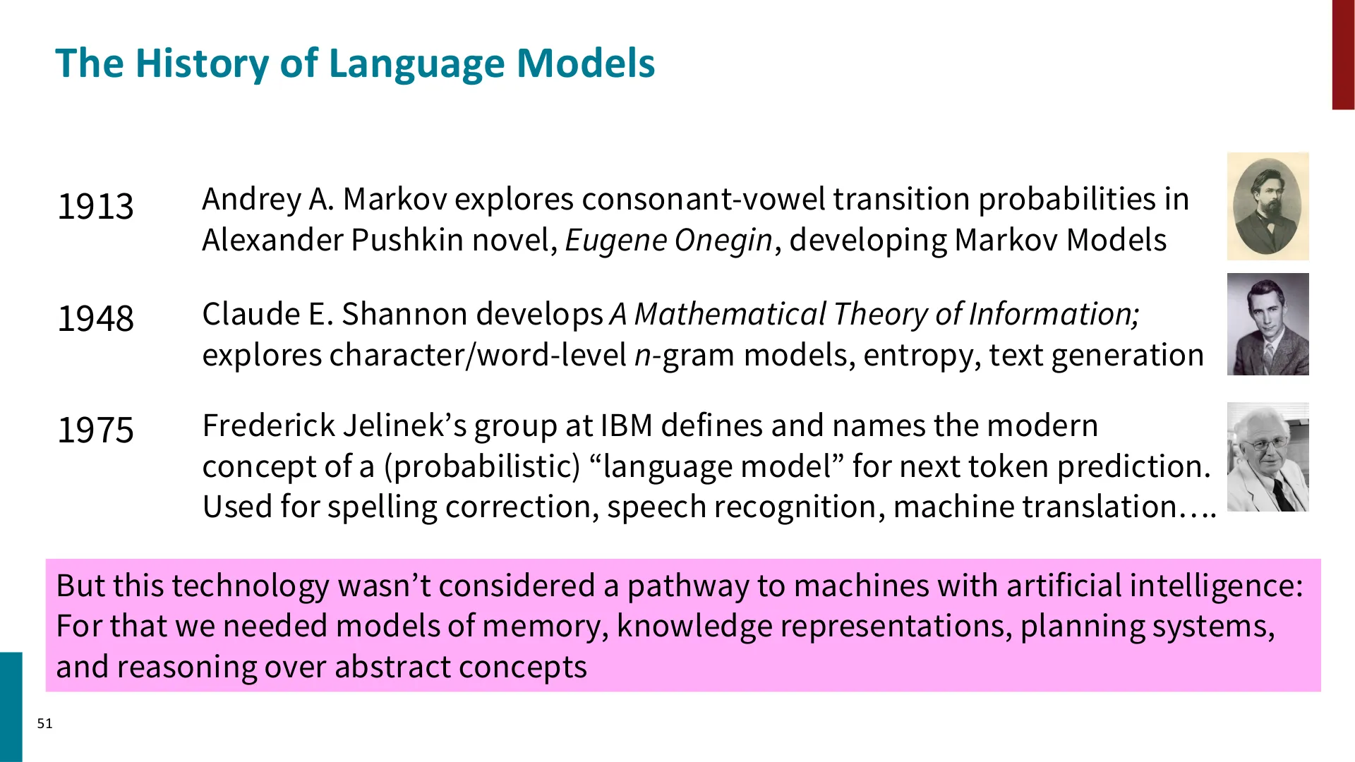
📷 The history of language models: Markov's character models (1913), Shannon's n-gram models (1948), Jelinek's probabilistic language models (1975)
回到原视频 (00:21:15)
Manning then points out why this is impressive, and his reasons are a checklist of what knowledge a language model must have absorbed:
- Cincinnati is in Ohio.
- In the United States, the Department of Energy regulates nuclear materials.
- If something is stolen, that is a theft, and agencies get involved.
- If it was a train carriage, then the train line, and where it runs, is relevant.
None of that is in the prompt. The model has it. And the output is not merely locally well-formed — the spelling is right, the sentences are real sentences rather than disconnected garbage — it is coherent discourse, a real story.
Editor's extension — the pre-history the slide puts behind language models. The slide dates the idea much earlier than 2019: Andrey Markov analysing consonant–vowel transitions in Pushkin's Eugene Onegin (1913); Claude Shannon's n-gram models, entropy and text generation in A Mathematical Theory of Communication (1948); and Frederick Jelinek's group at IBM defining and naming the modern, probabilistic language model for next-token prediction in 1975, used for spelling correction, speech recognition and machine translation. The slide's punchline is the crucial one for understanding the paradigm shift: for decades this technology was not considered a pathway to machines with artificial intelligence — for that, people thought, you needed models of memory, knowledge representation, planning and reasoning over abstract concepts. The paradigm shift was precisely the reversal of that judgement.
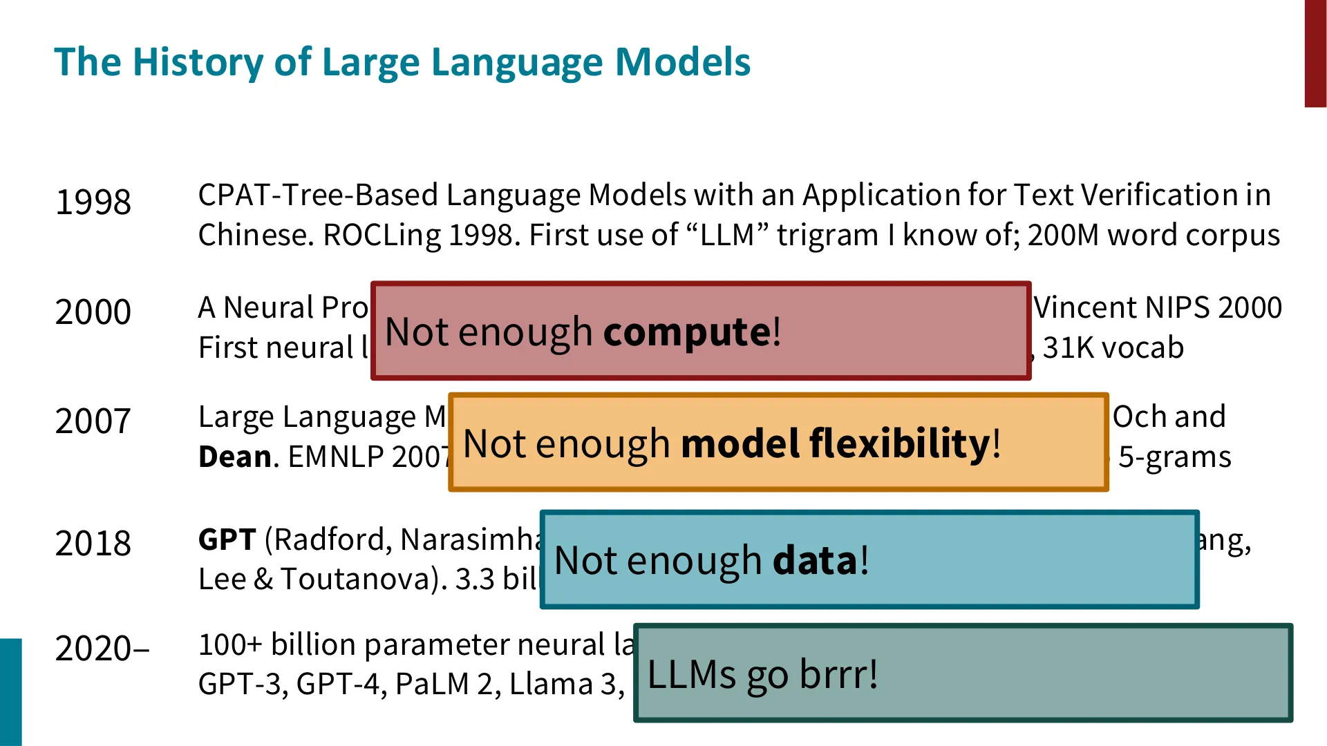
📷 The history of large language models: from a 1998 trigram "LLM" on a 200M-word corpus to 100+ billion-parameter models trained on more than a trillion tokens
回到原视频 (00:24:25)
(reference time: 00:24:20 — ChatGPT and GPT-4)
The next shift was a user-experience success, and Manning is emphatic that it mattered: with ChatGPT and GPT-4 you could ask questions or give commands, and the system would do what you wanted. His example is the kind of thing that made the system famous. He types a request to draft a polite email to his boss Jeremy saying he cannot come into the office for the next two days because his 9-year-old "song" is unwell — a misspelling of son — and that Peter is angry that he is not getting much attention. The system produces a sensible email, silently fixes the spelling mistake, and does not write about songs at all. Manning's comment is that the system works fine despite the typo, because it knows people make spelling mistakes.
(reference time: 00:25:15 — multimodality and foundation models)
Manning then widens the lens. Recent models are multimodal: they operate across modes, and you can ask them things like "what is unusual about this image?" The Stanford term for this generalisation, which he notes the group coined, is foundation models: the same technology applied across images, sound, bioinformatic signals such as DNA and RNA, seismic waves — "any kind of signal".
Text-to-image is the clearest demonstration. He asks for a picture of a train going over the Golden Gate Bridge (with a note for the Stanford Online audience who are not in the Bay Area: no trains go over the Golden Gate Bridge), and gets one. Then he iterates, and each iteration is a nice illustration of how the request is part of the model:
- The first image does not show the bay, so he asks for the bay in the background — and gets it.
- He wants a different style, so he asks for a detailed pencil drawing — and gets it.
- It is unrealistic for only trains to cross the bridge, so he asks for trains and cars — and gets both.
- With a newer model he escalates to a full scene: an illustration from a graphic novel, a bustling city street under a full moon, a young woman with fiery red hair in a velvet cloak haggling with a grumpy old vendor, and a tall sophisticated man in a sharp suit with a noteworthy moustache talking animatedly on a steampunk telephone.
His joke — that he made these artworks himself, so the audience should be impressed — is also the pedagogical point: the model follows a long, specific, compositional description, and the outputs are recognisably the same idea rendered in different styles.
Editor's extension — "foundation models". The term was introduced in On the Opportunities and Risks of Foundation Models (Bommasani et al., 2021) from Stanford's Center for Research on Foundation Models. The definitional move is exactly Manning's: one model, pretrained at scale on broad data, adapted to many downstream tasks and modalities — as opposed to one bespoke model per task.
Editor's note on the scale numbers. The two history slides give the numbers that make the "LLMs go brrr" transition concrete: a 1998 trigram "LLM" on a 200M-word corpus; Bengio et al.'s first neural language model in 2000 on 32M tokens with a 31K vocabulary; a 2007 n-gram model on a 2-trillion-token corpus; GPT-1 and BERT in 2018 on a 3.3-billion-token corpus; and 2020-onward models with 100+ billion parameters trained on more than a trillion tokens. The slide's annotations for the early years are "not enough compute", "not enough model flexibility", "not enough data" — the point being that the architecture did not change so much as the resources did.
6. From Denotational Semantics to WordNet: Why Dictionaries Fail a Computer
(reference time: 00:28:20)
Now the lecture turns to the technical core, starting with the question of what "meaning" is. Manning reads a dictionary definition: meaning is the idea represented by a word or phrase, the idea a person wants to express by using words. In linguistics, he says, the commonest way to think about this is as a pairing between a signifier (a symbol, a word) and a signified (an idea or thing). The technical name is denotational semantics: the idea or thing is the denotation of the symbol.
He notes that the same notion is used for programming languages. while, if and variables are symbols, and they have meanings — that is their denotation. And in natural language, the meaning of tree would be, roughly, all the trees you can find around the world.
Two things follow, and Manning is explicit about the second:
- This is a popular, perfectly reasonable notion of meaning, and it has never been very obvious what to do with it computationally.
- Pre-neural approaches therefore fell back on something much more primitive: looking at words and their relationships to one another.
The standard resource of that kind is WordNet, which he describes as a "sort of fancy thesaurus" that records word relations — synonyms and is-a (hypernym) relations:
- A panda is a kind of carnivore, which is a placental, which is a mammal.
- Good has multiple senses: a trade good, or the sense of goodness.
- You can explore the graph of these relations.
And then the problems, with a concrete example that sticks:
- Nuance is lost. WordNet will tell you that proficient is a synonym for good. But consider a sentence like "that was a good shot"—would you say "that was a proficient shot"? To Manning, that sounds weird. There is colour and nuance in how words are actually used that a relation graph cannot represent.
- Coverage is incomplete. Anything cooler, newer or slangier is missing — and it was already missing at the time, not just today.
- It is thoroughly human-made, with all the expense, inconsistency and staleness that implies.
The conclusion is the pivot of the entire lecture: can we represent meaning differently?
Editor's extension — how WordNet is organised, and why that structure is the problem. WordNet's unit is not the word but the synset: a set of near-synonymous words that share one sense (so bank appears in a financial synset and in a river-bank synset). Synsets are linked by semantic relations — hypernym/hyponym for
is-a, meronym/holonym for part-whole, antonymy, and so on. This is exactly what makes it good as a lexical database and bad as a computational model of meaning: it is discrete, sparse, expensive to extend, and it stores relations rather than degrees of similarity. There is no number in WordNet that says how similar two words are, which is precisely the number the next section sets out to learn.Editor's extension — why "proficient shot" is the right test case. Substitutability under synonymy is context-sensitive: good and proficient overlap in their denotation but differ in their selectional preferences and connotation (skill at a task vs. quality of an object or outcome). This is the first hint in the lecture that meaning has to be represented as something graded and context-dependent, not as a binary relation.
7. Word Vectors: Meaning as Numbers
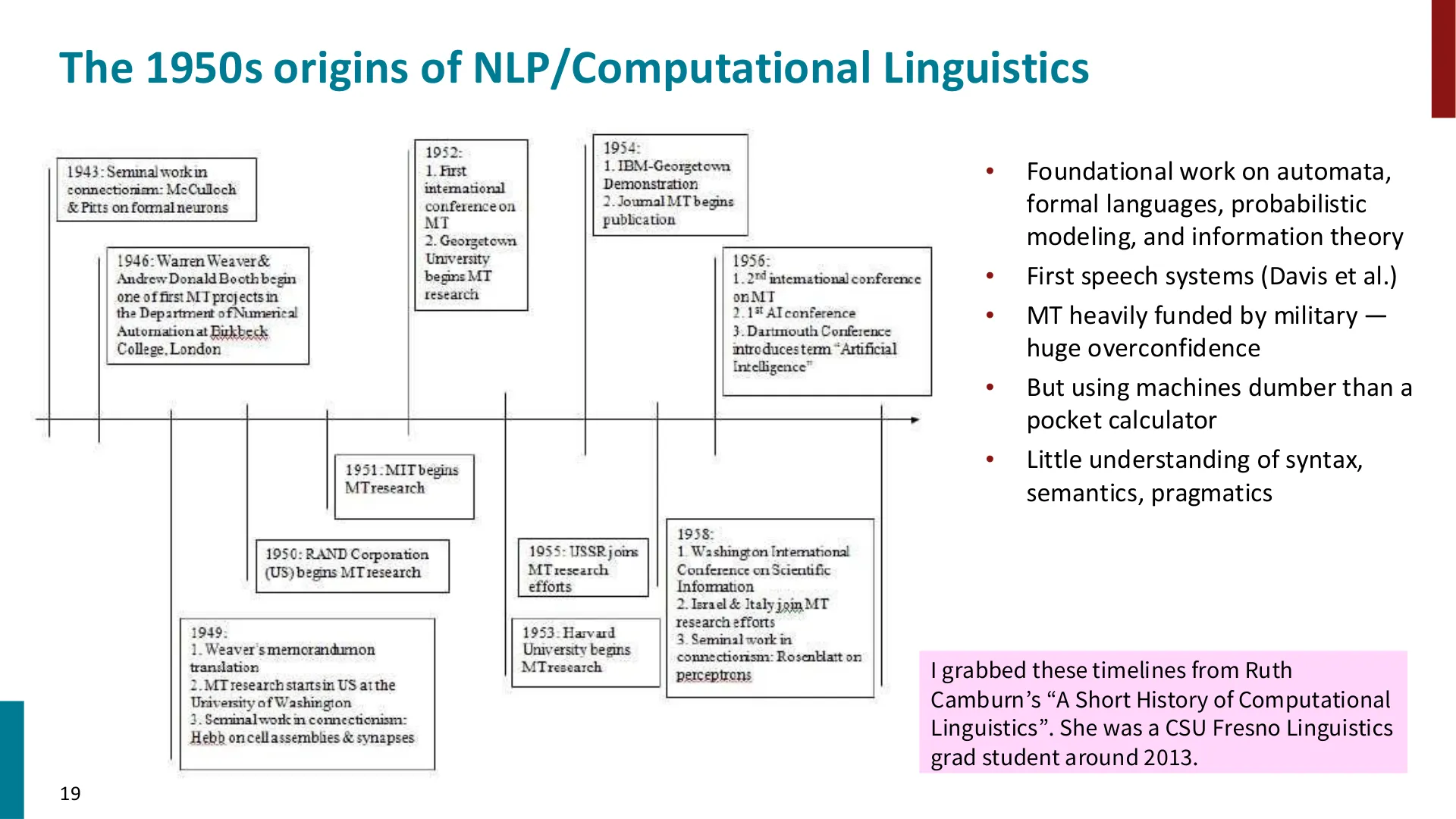
🖼️ Manning opens the deep-learning part by saying that language work began in the 1950s and had been struggling for sixty years; this page summarizes exactly what that early era achieved and got wrong (overconfident MT, weak hardware, little knowledge of syntax and semantics).
(reference time: 00:31:20)
The question is now concrete: when we have words like wicked, badass, nifty, wizard, what do they turn into inside a computer?
The starting point is that words are discrete symbols — atoms, essentially. The normal way to feed a symbol to a mathematical system is to give it an index in a vocabulary: motel is this entry in the vocabulary, hotel is that entry. Computational systems index strings to numbers, and the number gives the position in a vector. Since vocabularies are huge, so are these vectors: this is the one-hot vector representation, and Manning notes it was used for decades.
He then adds a term he had forgotten, going back two slides: these are localist representations — meaning that a word is represented at one single point. Here is where motel lives; here is where hotel lives.
(reference time: 00:32:45)
Why one-hot vectors are a poor way of computing with meaning:
- All words are equally unrelated. There is no inherent sense in which hotel and motel are close. They are two different symbols with a 1 in different positions.
- Formally, they are orthogonal and their dot product is zero. The two vectors have nothing to do with each other.
- People worked around this by building separate resources of word similarity and consulting them — in web search this was called query expansion — but the point stands: there is no natural notion of similarity inside a one-hot vector.
(reference time: 00:34:00)
The idea that follows is: what if we could learn to include similarity in the vectors themselves?
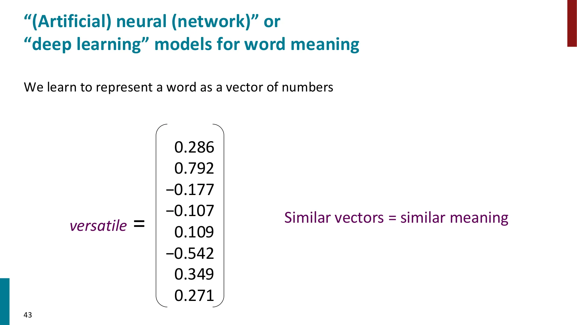
📷 Meaning as a vector of numbers: versatile = 0.286, 0.792, −0.177, …, with "similar vectors = similar meaning"
回到原视频 (00:36:25)
These are word vectors, also known as embeddings or neural word representations. Their properties, as Manning states them:
- They are short and dense — vectors of real numbers, not a vector as long as the vocabulary. The slide shows 8-dimensional vectors purely so they fit on a slide; in practice the length might be 200 or 2,000, compared with the half-million words in a vocabulary.
- Similarity is built in, expressed through the dot product. He walks through the arithmetic with banking and monetary: both are positive in the first dimension, both positive in the second, opposite in sign in the third and fourth. The dot product multiplies corresponding components and sums; it grows when components share a sign, and grows more when they are large in magnitude. So a large dot product means similar.
- They are called embeddings because we can think of each word as a point in a high-dimensional space, and the dimensionality of that space is the length of the vector.
(reference time: 00:38:15 — a warning about high-dimensional intuition)
Manning pauses on a point that beginners systematically get wrong. Humans cannot look at a 300-dimensional space or visualise what happens in it, so every picture he can show is two-dimensional — but high-dimensional spaces behave extremely differently from two-dimensional ones:
- In two dimensions, you are near to something else only if you are close in both x and y.
- In a high-dimensional space, a point can be near to all sorts of things along different dimensions at once.
That is exactly the property that lets a single vector capture several kinds of similarity and several senses of a word.
(reference time: 00:43:00 — student questions)
Three student questions here are worth keeping, because they are the questions beginners actually ask.
- How do you choose the dimensionality? Empirically or practically. Things start to work well around 100 dimensions; for a long time people used 300 because it seemed to work pretty well; as models and datasets got much larger, 1,000 or even 2,000 dimensions became increasingly common.
- Are the entries bounded between −1 and 1? They do not have to be, and with the way these vectors are learned they are not bounded. You can bound them: sometimes people length-normalise so that vectors have length one. In general, regularisation is used to keep coefficients from getting huge.
- Do we only use distance, or also direction? Not only distance — directions in the space carry semantic meaning too, and he promises an example shortly.
The first question about context arrives here as well, and Manning's answer defines the scope of the lecture: for now, the model learns one vector per string of letters. So star gets a single vector, and it will not distinguish a Hollywood star from an astronomical star. What it will do is sit close to astronomical words such as nebula and, simultaneously, close to words like celebrity. The details of that are the last section of this book, and the contextual representations that fix it come later in the course.
Editor's extension — one-hot, localist, distributed. The contrast Manning draws is the classic localist vs. distributed distinction. A localist code devotes one unit to one concept, so $n$ concepts need $n$ units and any two codes are orthogonal: $\text{motel} \cdot \text{hotel} = 0$. A distributed code spreads one concept over many units and reuses those units across concepts, so $n$ concepts can be represented with far fewer than $n$ units, and similarity becomes a computable quantity — the dot product of two codes. Everything interesting later in the course (weight tying, softmax over a vocabulary, cosine similarity between sentence representations) depends on this change of representation.
Editor's extension — dot product vs. cosine similarity. The dot product grows with the magnitudes of the vectors as well as with their alignment. Cosine similarity, $\cos(u,v) = \frac{u \cdot v}{\lVert u \rVert \lVert v \rVert}$, removes the magnitude and measures only direction. This is why length-normalising vectors (the student's question above) is such a common operation: it turns "large dot product" into "same direction", which is usually what you want when you ask whether two words are similar.
8. Distributional Semantics: Meaning from the Company a Word Keeps
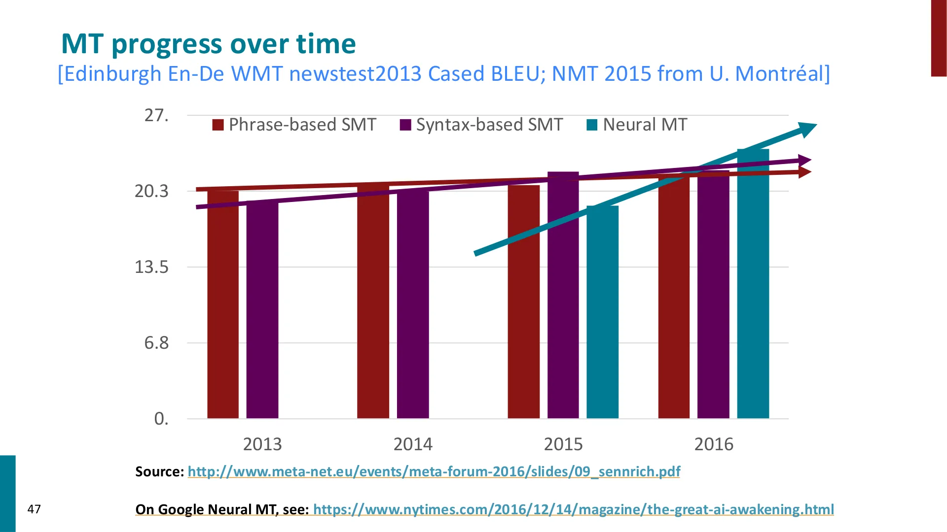
🖼️ The chart shows the jump from phrase-based and syntax-based SMT to neural MT between 2013 and 2016, the exact evidence behind Manning's claim that neural MT was so good it was commercially deployed almost immediately.
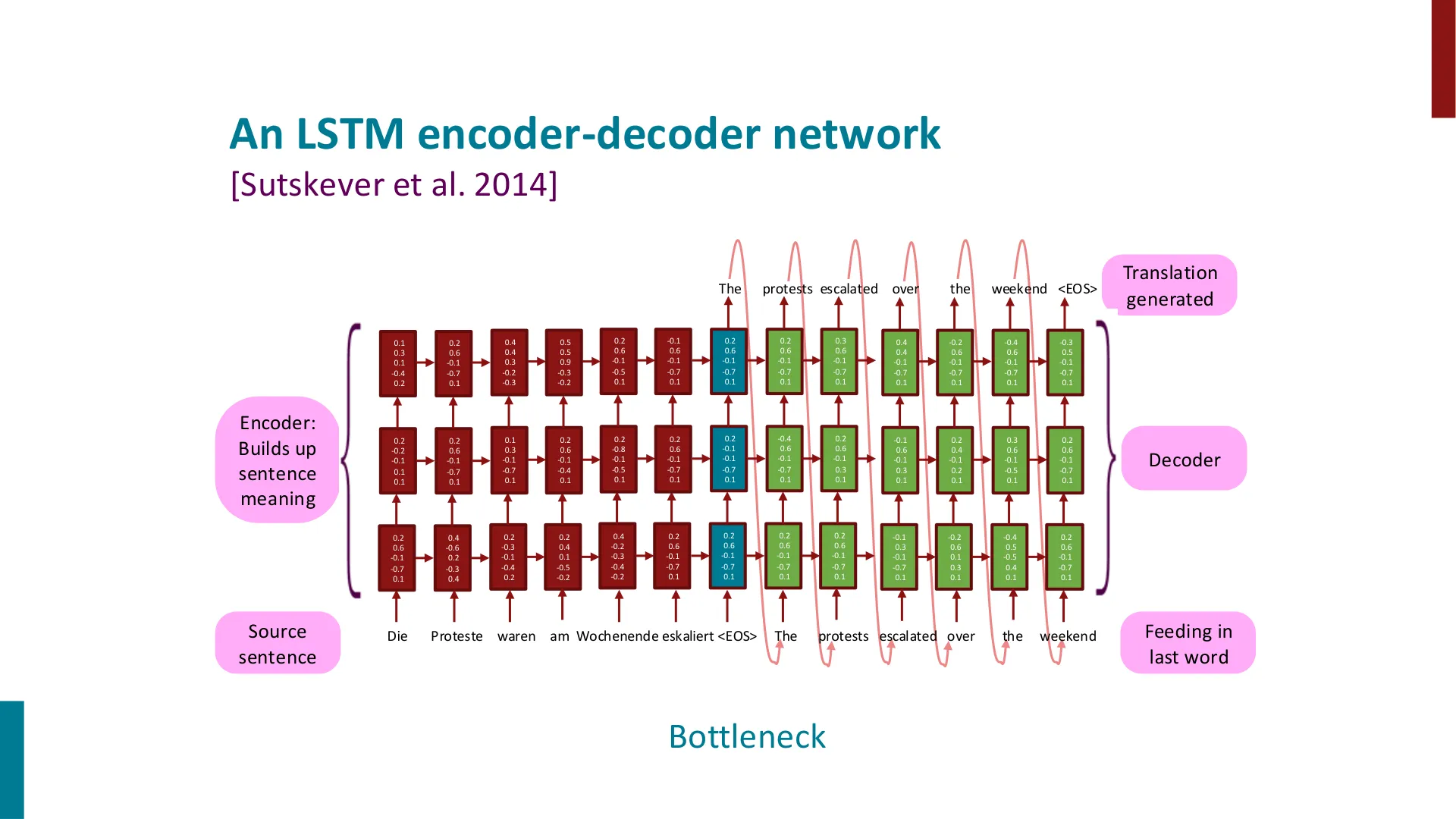
🖼️ This is the encoder-decoder figure with the labels Manning uses in words - the encoder builds up sentence meaning, the decoder generates the translation and is fed the last word - including a concrete German-to-English example.
(reference time: 00:34:55)
There is an older idea about meaning that the word-vector approach is really an implementation of. Manning quotes the line everyone quotes, from the British linguist J. R. Firth (1957):
"You shall know a word by the company it keeps."
The idea goes back further, to philosophical work by Wittgenstein and others: represent a word's meaning by the contexts in which it appears. The words that occur around a word carry information about its meaning. This is distributional semantics, in contrast to the denotational semantics of the previous section.
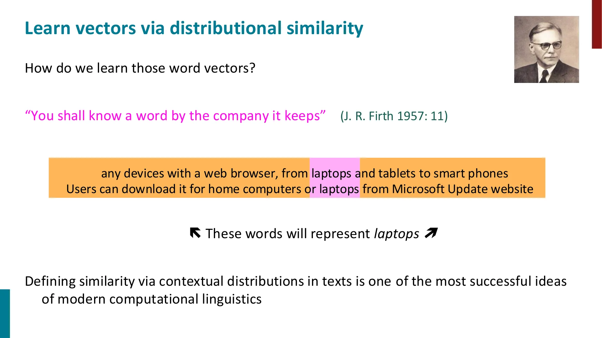
📷 Firth's "You shall know a word by the company it keeps", with the laptop-context example that introduces distributional semantics
回到原视频 (00:35:05)
Concretely, if we want to know about the word banking, we collect sentences that use it — his example is the kind of financial-news sentence in which "government debt problems turned into banking crises, as happened in 2009". The words that occur around banking in such sentences — debt, problems, crises, government — become the meaning of banking.
So the plan is:
- Take statistics about which words appear near which other words in a corpus.
- Use those statistics to learn a new kind of representation: a short, dense vector that captures the meaning of the word.
(reference time: 00:39:00 — what the learned space looks like)
The predicted payoff is a geometric one: if two words have something to do with each other, they will end up with similar vectors, i.e. a large dot product. Two-dimensional projections of such a space are the famous pictures in NLP courses, and Manning zooms into two regions to show that the structure is not just "clusters of unrelated words" but genuinely interpretable:
- A region of country and location words, with nationality terms such as British, Australian, American, European nearby.
- A region of verbs, with fine structure:
- verbs of communication, statement and thought — saying, thinking, expecting — grouped together;
- come and go grouped together;
- forms of have lower down;
- forms of be above them;
- and become and remain close to be, because they take the same kind of complement of state: just as you can say "I am angry", you can say "he remained angry" or "he became angry".
So the space really does have semantic structure: things with similar meaning are close together, and the neighbourhoods are informative. The remaining question — and the technical content of the lecture — is how we get there.
(reference time: 00:43:20 — student question about the pictures)
A student asks how a high-dimensional space is brought down to a low-dimensional one for visualisation. The pictures use t-SNE, a non-linear dimensionality reduction method that tends to work better for high-dimensional neural representations than PCA, which is more familiar from other courses.
Editor's extension — what t-SNE does, and what it does not. t-SNE (van der Maaten & Hinton, 2008) places points in two dimensions so that the neighbourhood structure of the original space is approximately preserved: points that were close stay close, and points that were far apart are pushed apart. Two caveats matter when reading the pictures above. First, distances between clusters in a t-SNE plot are not meaningful — only neighbourhoods are. Second, the method is stochastic, so different runs give different-looking pictures of the same space. Do not read a t-SNE plot as a map with a scale.
Editor's extension — prediction test. Notice what the objective will actually be: predict context words from a center word, not merely count co-occurrences. This is the crucial difference between the classical distributional-semantics literature (count, then reduce, e.g. by SVD) and the neural approach taught here (learn the vectors by gradient descent on a prediction task). The lecture makes the same point implicitly when it says the vectors are the parameters of a predictive model.
9. Word2vec: Learning Vectors by Predicting Nearby Words
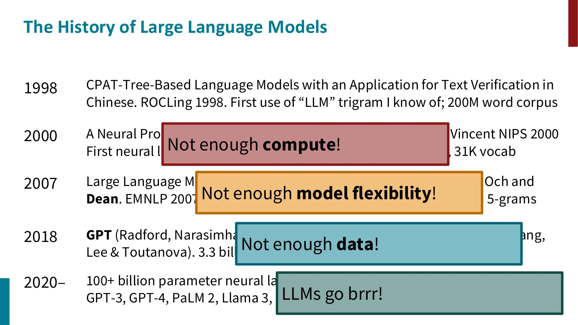
🖼️ The annotated timeline of large language models (1998 to 2020+) shows the scale of data and models behind the GPT-2 and ChatGPT discussion, including the annotated bottlenecks on compute, model flexibility and data.
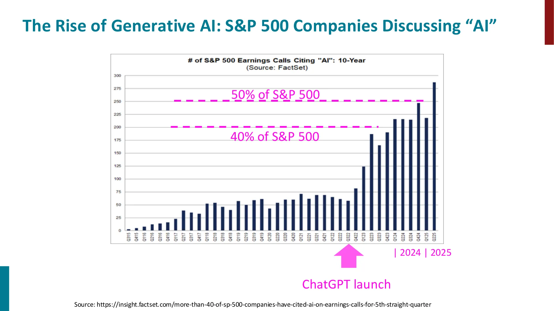
🖼️ Manning stresses that ChatGPT was a huge user success and that the whole world started talking about AI; this page marks the ChatGPT launch and the surge of AI discussion among S&P 500 companies.
(reference time: 00:47:12)
Manning now introduces the algorithm that the rest of the lecture is about. word2vec was devised by Tomáš Mikolov and colleagues at Google in 2013. Three things about its status:
- It was not the first method for learning word vectors — others go back to around the turn of the millennium.
- It was not the last either; others came after it.
- But it was particularly simple and particularly fast, and that is what caught people's attention.
9.1 Corpus, word type, and the sliding window
(reference time: 00:47:45)
The input is a large amount of text: just a long list of words. In NLP this is called a corpus — Latin for "body". Manning pauses here for a joke that is worth preserving because it also makes the term memorable: yes, corpus is exactly the same word as the Latin for a body lying on the floor, but we mean a body of text. And, since classical education is not what it used to be, a piece of morphology: corpus, despite the -us ending, is a fourth-declension neuter noun, so its plural is not "corpys" — it is corpora. He adds that sooner or later he will read a project assignment that refers to "corpys", and that person will have demonstrated they were not paying attention in the first lecture.
Two more definitions, used carefully throughout:
- A word type is a word as a vocabulary item — star, bank, wherever it occurs.
- A word token is one particular instance of that word in a text.
The algorithm learns one vector per word type.
The mechanical setting:
- Go through every position in the text.
- At each position there is a center word $c$ and the words outside it, within a fixed window of size $m$ (in the example, $m = 2$, i.e. two words to the left and two to the right).
- Use the similarity of the vectors for the center word and the outside words to compute the probability that those outside words occur near the center word — and make that probability as high as possible on the observed data.
His concrete example is a fragment in which the words problems turning into banking crises appear, and the question the model must answer is how likely it was that turning occurred before into, and so on for the words in the window around each position. The model is obviously not going to be able to answer such questions well — seeing banking does not tell you that into will occur — but Manning's standard is modest and precise: after the word banking, crisis should be pretty likely and skillet should not be. Getting that right is doing a good job.
9.2 From likelihood to an objective function
(reference time: 00:52:00)
Turning the idea into mathematics takes three steps, each of which he justifies as a matter of convenience:
- Maximise a likelihood. Over every position in the corpus, and every word in its context window, we want the probability of the observed context words to be as high as possible:
$$L(\theta) = \prod_{t=1}^{T}\ \prod_{\substack{-m \le j \le m \\ j \ne 0}} P(w_{t+j} \mid w_t)$$
- Put a minus sign in front. "For completely arbitrary reasons — it really makes no difference — everyone got into minimizing things rather than maximizing things." The algorithms are therefore called gradient descent, and we work with a negative log-likelihood.
- Take the logarithm. Working with a huge product is harder for the math; but the log of a product is a sum. So instead of multiplying many probabilities, we sum many log-probabilities.
Finally, since the sum would otherwise grow with the length of the corpus, he divides by the number of words, giving the objective:
$$J(\theta) = -\frac{1}{T}\sum_{t=1}^{T}\sum_{\substack{-m \le j \le m \\ j \ne 0}} \log P(w_{t+j} \mid w_t)$$
This is the average negative log likelihood, and minimising it maximises the probability of the words in context.
9.3 The only parameters are the word vectors
(reference time: 00:54:50)
The next trick defines the probability that the model is maximising. Each word type is represented by a vector of real numbers — say 100 of them — and the probability is computed only from those vectors. Manning is explicit that this means the model's parameters, $\theta$, are nothing but the word vectors for every word in the vocabulary. That is a lot of parameters, but there is nothing else.
The probability of an outside word $o$ given a center word $c$ is defined in terms of the dot product of the two vectors:
$$P(o \mid c) = \frac{\exp\!\left(u_o^\top v_c\right)}{\sum_{w=1}^{V}\exp\!\left(u_w^\top v_c\right)}$$
High dot product means high co-occurrence probability. Manning adds an honest caveat about what "similar" means here. Yes, we want hotel and motel to be similar. But we also want the word the to be able to appear easily before student — so in this weird sense the also has to be similar to student, and in fact to basically any noun. This is a hint of how crude the model is: it is a single vector per word, and the "similarity" being learned is a similarity of co-occurrence, not of lexical meaning.
9.4 Two vectors per word
(reference time: 01:02:30)
One more design detail, which he flags as making the math a little simpler: each word gets two vectors — one used when the word is the center word $v_c$, and one used when it is an outside word $u_o$. He promises to explain the benefit later, and the benefit shows up in the derivation, where it makes the gradient take a clean form.
The parameter count is then easy to compute, and he does compute it, because it shows the scale of what is being optimised. With 100-dimensional vectors and a vocabulary of 400,000 words:
$$400{,}000 \times 2 \times 100 = 80{,}000{,}000 \text{ parameters}$$
Eighty million parameters to fiddle with. "Luckily, we have big computers."
graph TD
    A["Corpus: a long list of words"] --> B["Slide a window of size 2m+1 over every position"]
    B --> C["Center word c, outside words o within m"]
    C --> D["Score each pair: u_o^T v_c"]
    D --> E["Softmax over the whole vocabulary"]
    E --> F["Objective J: average negative log likelihood"]
    F --> G["Compute the gradient of J with respect to every vector in theta"]
    G --> H["Take a gradient descent step: update all vectors"]
    H -->|next position| B
Editor's extension — which word2vec is this? The derivation in this lecture is the skip-gram variant with a full softmax: predict context words from a center word, normalising over the whole vocabulary. The original paper introduces both skip-gram and CBOW (predict the center word from its context), and the companion paper introduces negative sampling, which replaces the expensive normalisation with a binary discrimination task. The lecture never names the variant, but the objective written on the slide — a sum over context words of log-softmax probabilities — is skip-gram.
Editor's extension — why a full softmax is too expensive to be practical. The denominator sums over all $V$ vocabulary words for every single training pair, so the cost per step is proportional to the vocabulary size. This is exactly the computational problem that negative sampling and hierarchical softmax were invented to solve, and it is the reason the definition of the probability in this lecture is pedagogically clean but not what you would run on a large corpus. If you build this model yourself, this is the line you will want to change.
10. Softmax: Turning Similarities into Probabilities
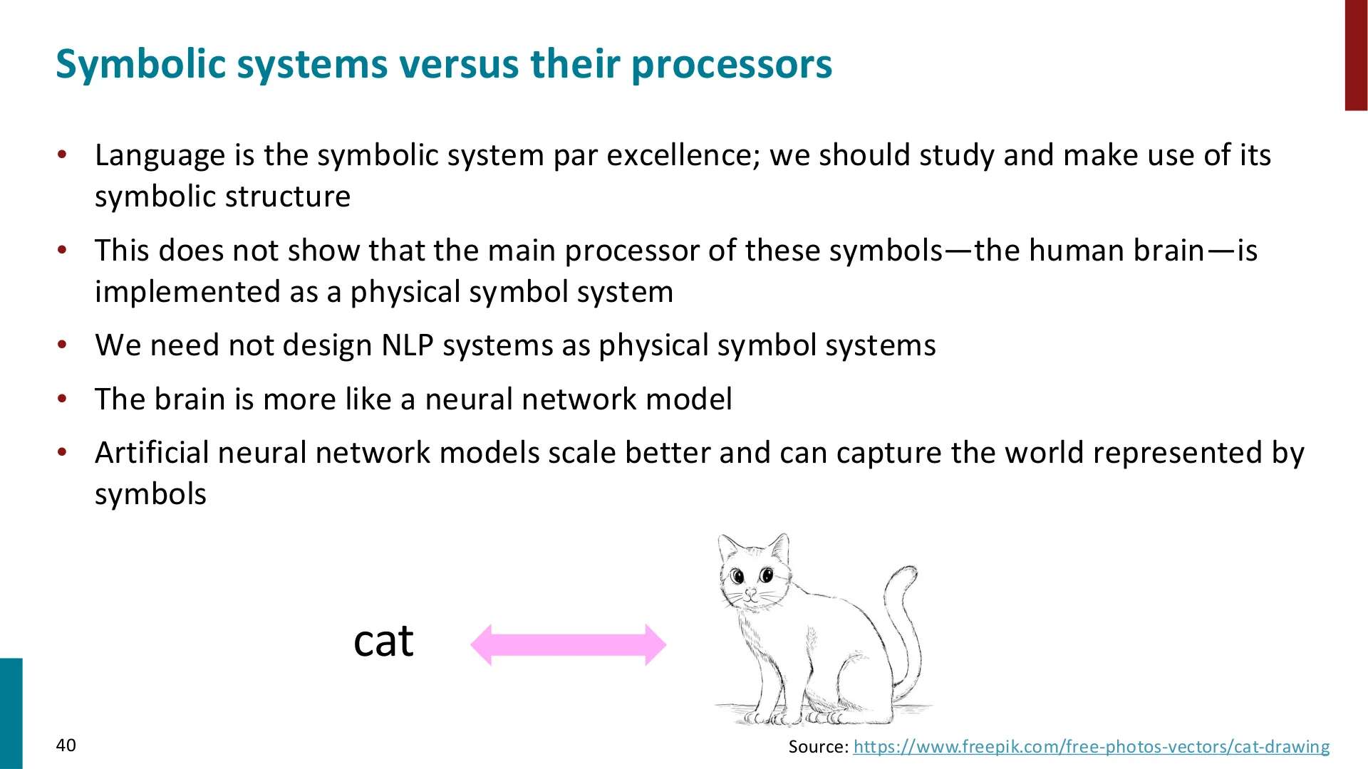
🖼️ This page makes exactly the argument Manning builds toward: language is the symbolic system par excellence, but the brain is more like a neural network model and artificial neural networks scale better while capturing the world represented by symbols - the bridge from denotational semantics to vectors.
(reference time: 00:56:50)
The formula in the previous section deserves to be unpacked, because it is the tool the entire course will keep reusing.
Start from the dot product $u_o^\top v_c$:
- You multiply each pair of corresponding components and sum the results.
- If the two components have the same sign, that contributes positively; if they are both large in magnitude, it contributes a lot.
- So the dot product is a measure of similarity — but it is an unbounded real number, free to be negative or positive.
We want a probability out of it. Three steps get us there:
- Exponentiate. $e^x$ is positive for any real $x$, so the exponential guarantees non-negativity.
- Normalise. Compute that quantity for every possible context word, sum them all, and divide by the total — "the dumbest way possible" to turn positive numbers into numbers between 0 and 1.
- Read off a distribution. The result is a probability distribution over context words that sums to 1 by construction.
$$\text{softmax}\!\left(u_o^\top v_c\right) = \frac{\exp\!\left(u_o^\top v_c\right)}{\sum_{w=1}^{V}\exp\!\left(u_w^\top v_c\right)}$$
This is the softmax function. Manning explains the name carefully, because beginners find it unintuitive:
- It amplifies the largest values, because of the exponential — this is the "max" part.
- But it is soft, because smaller items still receive some probability, rather than being discarded — unlike a true
max, which picks out exactly one thing. - So the name is "sort of a funny name": softmax turns a bunch of unbounded real numbers into a probability distribution, approximating a maximisation without committing to it.
The closing remark generalises the tool: softmax is used everywhere in deep learning — any time you have vectors in $\mathbb{R}^n$ and want probabilities, you shove them through a softmax.
graph LR
    A["Dot product u_o^T v_c<br/>any real number, possibly negative"] --> B["Exponentiate<br/>exp(u_o^T v_c) is always positive"]
    B --> C["Normalise<br/>divide by the sum over all V vocabulary words"]
    C --> D["Probability distribution over context words<br/>sums to 1 by construction"]
Editor's note on numerical practice. Exponentiating unbounded scores is fine mathematically and dangerous numerically: if a dot product is large,
expoverflows. Real implementations subtract the maximum score before exponentiating — the same distribution results, because the constant cancels in the numerator and denominator — and this shift-max trick is standard in every deep-learning framework. You will see it in HW2 and HW3.
11. Training: The Objective, the Gradient, and Gradient Descent
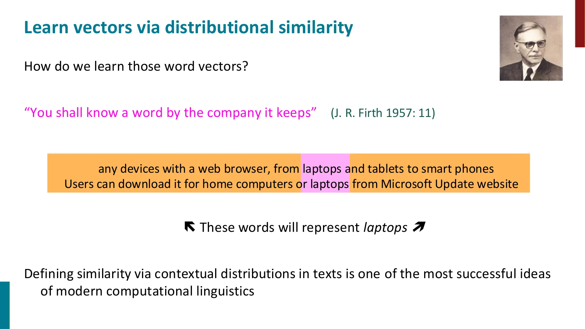
🖼️ The Firth quote - you shall know a word by the company it keeps - is exactly the quotation Manning uses when he introduces distributional semantics, and the page shows how shared context words give laptops its meaning.
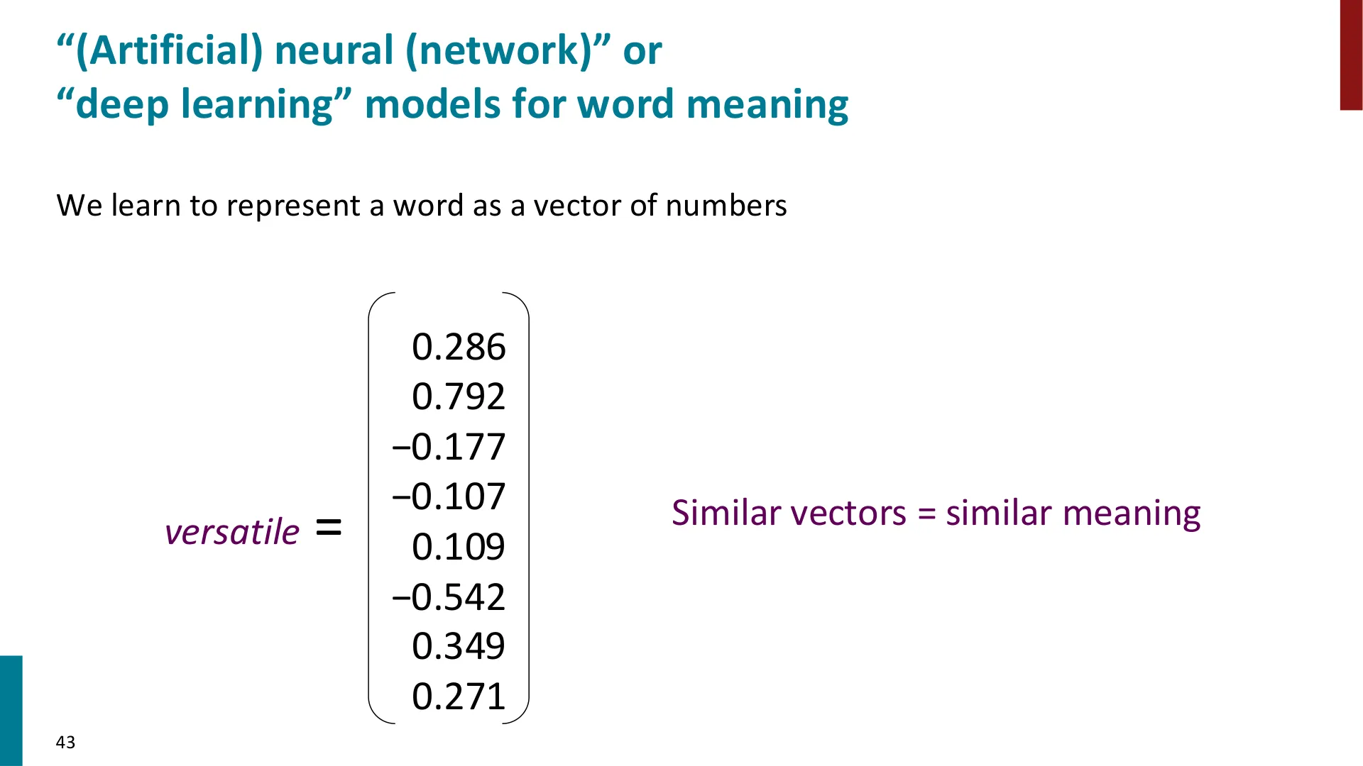
🖼️ This is the central idea of the section in one picture: a word such as versatile becomes a vector of numbers, and similar vectors mean similar meanings.
(reference time: 01:00:00)
The picture is now complete except for the crucial question: where do the vectors come from? Manning's answer is that we turn the whole thing into an optimization problem:
- Start with random vectors for every word.
- Fiddle with them so that the calculated probabilities of the observed context words go up.
- Keep fiddling until they stop going up — that is, until the probability estimates are as high as we can get.
- The fiddle is done with calculus: compute the derivatives of the objective with respect to every parameter.
(reference time: 01:01:30 — the two-dimensional intuition)
He gives the standard picture, and it is worth keeping because it is the only intuition many students will carry into higher dimensions. In a two-dimensional space, if you want to find the minimum and you start at the top left, you compute the derivatives there; they point down and a little to the right, so you walk down and a little to the right. At the new place, compute the derivatives again; they still point downhill; walk again. Keep walking and you reach the minimum.
In this model there are far more than two dimensions: the parameters are the concatenation of all the word vectors — and, as established, twice the vocabulary, because each word has a center vector and an outside vector. He sketches the parameter space as the list of vectors from aardvark as an outside word, through the vocabulary, to zebra as an outside word, and then the center vectors after that: 80 million numbers in the earlier example. We compute gradients for all of them.
And then a remark that is worth preserving verbatim in spirit, because it is the "magic" that the rest of the quarter will explain: it does not seem like it should work. You start with nothing — random word vectors and a pile of text — do some math, and get something useful out. But that is what happens in these deep-learning optimisation problems.
(reference time: 01:04:50 — the derivation, done slowly on purpose)
Before starting the calculus, Manning addresses the audience directly, and the aside is part of the pedagogy: many students taking CS224N already know much more math than he does, so the next ten minutes may be extremely boring for them — they can catch up on Discord or Instagram, or leave. But other students taking CS224N cannot quite remember when they last took a math course, and he wants everybody to be able to learn something, which is why in the first two weeks he goes through this concretely.
The objective, restated. The negative average log-likelihood of the context words over the corpus (Section 9.2), with $\theta$ standing for all the word vectors.
The probability, restated. The softmax of the dot product of an outside vector and a center vector, normalised over the vocabulary (Section 10).
The derivative we want. The partial derivative of the objective with respect to the center word vector $v_c$ (the outside-word parameters can be done separately, and in the event there is no time for them). Because the objective is a big sum of terms, and the derivative of a sum is the sum of the derivatives, we can work one term at a time.
Step 1: split the logarithm. The term is a logarithm of a quotient, and the log of a quotient is the difference of logs:
$$\frac{\partial}{\partial v_c}\log P(o\mid c) = \frac{\partial}{\partial v_c}\log \exp\!\left(u_o^\top v_c\right) - \frac{\partial}{\partial v_c}\log \sum_{w=1}^{V}\exp\!\left(u_w^\top v_c\right)$$
Step 2: the easy half. In the numerator, $\log$ and $\exp$ are inverse functions, so they cancel, leaving $u_o^\top v_c$. Its derivative with respect to $v_c$ is $u_o$. He does not just assert this; he shows why on a component:
$$u_o^\top v_c = u_1 v_1 + u_2 v_2 + u_3 v_3 + \dots$$
Taking the partial derivative with respect to $v_1$ kills every term except the first, leaving $u_1$; with respect to $v_2$, leaving $u_2$; and so on. Walking along the whole vector, the answer is the vector $u$ — "that part is easy."
Step 3: the hard half, and the chain rule. The denominator is a function inside a function: an inner function of $v_c$ whose output he calls $z$, and an outer function (the logarithm). The chain rule says to take the derivative of the outer function with respect to $z$, times the derivative of $z$ with respect to $v_c$. The derivative of $\log$ is $1/x$ — "you have to remember that, or look it up, or get Mathematica to do it for you" — so:
$$\frac{\partial}{\partial v_c}\log \sum_{w=1}^{V}\exp\!\left(u_w^\top v_c\right) = \frac{1}{\sum_{w=1}^{V}\exp\!\left(u_w^\top v_c\right)} \cdot \frac{\partial}{\partial v_c}\sum_{w=1}^{V}\exp\!\left(u_w^\top v_c\right)$$
Step 4: chain rule again, inside the sum. The sum can move outside the derivative. Each term is again a function inside a function: the exponential outside, and the dot product inside. The derivative of the exponential is the exponential itself, so:
$$\sum_{w=1}^{V}\ \exp\!\left(u_w^\top v_c\right) \cdot \frac{\partial}{\partial v_c}\left(u_w^\top v_c\right) = \sum_{w=1}^{V}\exp\!\left(u_w^\top v_c\right)\cdot u_w$$
using the derivative of the dot product that was worked out in step 2.
Step 5: put the two halves back together. The numerator derivative is $u_o$; the denominator derivative is the sum above, over the denominator. Combining them:
$$u_o - \frac{\sum_{w=1}^{V}\exp\!\left(u_w^\top v_c\right) u_w}{\sum_{w=1}^{V}\exp\!\left(u_w^\top v_c\right)} = u_o - \sum_{x=1}^{V} P(x\mid c)\,u_x$$
because the ratio in the middle is exactly the softmax from Section 10.
(reference time: 01:18:00 — what the result means)
Manning stops to interpret the formula rather than just admire it, and this is the part to remember:
- The gradient is the observed vector minus a weighted average of all the vectors, where the weights are the model's current softmax probabilities.
- The quantity being subtracted is the model's expectation: if the model is currently assigning high probability to some word $x$, that word's outside vector gets a large weight in the average.
- The shape "observed − expected" recurs constantly in derivatives of this kind.
- What you want is for the weighted average — the expectation — to equal what was observed, because then the derivative is zero and you have reached a maximum.
For the full objective you also need the derivatives with respect to the outside vectors, but "hey, it's officially the end of class time", so he wraps up: we work out all of these derivatives for every parameter, those derivatives give a direction in which to change the numbers, and that lets us find good word vectors automatically. His final reassurance is the practical one: he wants students to understand how this works, but they will find out very quickly that computers do it for you, and they will not have to do it by hand on a regular basis. More on that on Thursday.
(The derivation was written out by hand on an iPad during the lecture, and Manning comments in the middle that the handwriting is not going well — the tidy version he prepared at home is on the slides on the website. The book reproduces the tidy version.)
graph TD
    A["Initialise all word vectors randomly"] --> B["Compute J(theta) over the corpus"]
    B --> C["Compute the gradient of J with respect to every parameter"]
    C --> D["Take a step in the downhill direction"]
    D --> E{"Is the likelihood still improving?"}
    E -->|yes| B
    E -->|no| F["Stop: the current vectors are the learned word vectors"]
Editor's note on the minus sign. Strictly, the quantity derived above is the derivative of the log-likelihood, and its zero point is a maximum of the likelihood — which is exactly how Manning describes it at the end. The objective $J$ actually minimised is the negative average log-likelihood, so its gradient is the negative of this expression, and gradient descent therefore moves the parameters in the direction that increases the probability of the observed context. Nothing in the derivation changes; only the sign of the step.
Editor's extension — why "observed − expected" is such a good sign. This form is a fixed point of the learning dynamics: training stops (for that term) precisely when the model's predicted distribution matches the data. It is the same algebraic shape that appears in logistic regression, in the EM algorithm's M-step, and in the gradients of much larger sequence models. Recognising it once means recognising it everywhere.
Editor's extension — why two vectors per word helps. With separate $u$ (outside) and $v$ (center) vectors, the gradient with respect to $v_c$ involves only the $u$ vectors, and the gradient with respect to $u_o$ involves only the $v$ vectors. The two parameter sets do not appear multiplied together inside the gradient of a single term, which keeps each update simple. In practice, once training is finished the two matrices are often combined — most commonly by adding or averaging them — to give one vector per word.
12. Summary: What Static Word Vectors Achieve, and What They Miss
The lecture's last technical thread is the limitation that has been visible since Section 7, and Manning states it plainly.
One word type, one vector. For now, the algorithm learns a single vector for each string of letters, and that vector does not capture the meaning of a word in context. Hence:
- star will not distinguish the Hollywood sense from the astronomical sense. What happens instead is that its single vector ends up close to astronomical words such as nebula and simultaneously close to words for a Hollywood star. When he asks the room for such a word, a student offers celebrity — and the fact that this is easy for humans to supply is the whole point.
- bank is the same story: a financial institution or a river bank. The learned vector behaves like an average over its senses, which is why it ends up near words that are semantically evoked by both senses.
The average is still useful, and that is why the method works. In a high-dimensional space (Section 7), a point can be close to different groups along different dimensions, so a single vector can serve several senses well enough to be worth having. The multi-sense problem is real, but it does not make one-vector-per-word useless.
What comes next, and why this is the interesting part. To represent word meaning in context you need contextual representations. That is the subject of the rest of the course: recurrent networks, attention, Transformers, and pretrained models. The student question from Section 7 — "doesn't similarity depend on context?" — was correct, and it was deliberately deferred: "that's a good thought, you can keep it for a few weeks".
The second takeaway of the lecture is methodological, and it is the one to carry into the assignments. Starting from random vectors and a pile of text, and doing nothing but optimisation, produced a representation with genuine semantic structure — countries near countries, thought-verbs near thought-verbs, become and remain near be. That is the first concrete example of the "magic" that deep learning keeps performing, and it is why the course insists on the word2vec derivation rather than treating it as a black box.
Editor's note — what did not happen in this recording. Manning opened by saying he hoped to spend a few minutes at the end playing with a Jupyter notebook to show what these word vectors can do, and admitted at 01:04:30 that he would probably not get to the end of what he hoped for. He did not: there is no notebook walk-through in this video, and the derivatives with respect to the outside vectors were left for the next lecture.
附:官方参考与延伸阅读
Course material
- Course website: cs224n.stanford.edu — syllabus, slides, assignments, office hours, Ed discussion board. Assignments are submitted via Gradescope through Canvas.
- Slide decks used for this lecture:
cs224n-2026-lecture01-history.pdf(the four eras, the 1950s–2010s history, machine translation, the history of language models) andcs224n-2026-lecture01-intro.pdf(course logistics, learning goals, assignments, lecture plan). Both were provided with the recording; slide PDFs are posted before each lecture on the course site. - Course plan quoted in the decks: Lecture 1 — Introduction and the History of NLP, with the stated key learning: "understand the paradigm shifts in NLP and how our assumptions about language shape what is possible in each era."
- Licensing: the material provided with this recording did not include a licence statement for the slide decks; the decks appear to be protected course material. Slide titles are quoted here only as short pointers to the figures reproduced for commentary. See Known Uncertainties.
- "A creative way of looking at the history of NLP": a physical exhibition by the Stanford NLP group in Gates Building, room 3B (credited on the slides).
Sources behind the history section (Chapter 3 and the history slides)
- Christopher D. Manning, Human Language Understanding & Reasoning, Dædalus 151(2): 127–138, Spring 2022 — amacad.org/publication/human-language-understanding-reasoning. Source of the four-era framing and of the judgement that NLP and AI/nets are "only somewhat entwined fields".
- Warren Weaver (1955, quoting a 1947 letter) on translation as decoding — quoted on the history slides.
- Norbert Wiener's 1947 reply doubting quasi-mechanical translation because the semantic boundaries of words differ across languages — same slides.
- McCulloch & Pitts (1943), "A Logical Calculus of Ideas Immanent in Nervous Activity" — background article: nautil.us/the-man-who-tried-to-redeem-the-world-with-logic-235253.
- Frank Rosenblatt and the Mark I Perceptron — Cornell news feature.
- Vannevar Bush (1945), "As We May Think", The Atlantic — theatlantic.com/magazine/archive/1945/07/as-we-may-think/303881. The origin of the "memex" and of information retrieval.
- Claude E. Shannon (1948), A Mathematical Theory of Communication — background article: quantamagazine.org/how-claude-shannons-information-theory-invented-the-future-20201222.
- The 1958 New York Times article "New Navy Device Learns by Doing", reproduced on the history slides, is the canonical example of early AI hype.
Word meaning, word vectors, word2vec
- J. R. Firth (1957), "You shall know a word by the company it keeps" — quoted on the slides; the origin of distributional semantics.
- George A. Miller et al., WordNet, Princeton — the lexical database discussed in Chapter 6.
- L. van der Maaten & G. Hinton (2008), Visualizing Data using t-SNE, JMLR 9 — jmlr.org/papers/v9/vandermaaten08a.html.
- T. Mikolov et al. (2013), Efficient Estimation of Word Representations in Vector Space — arxiv.org/abs/1301.3781. Introduces CBOW and skip-gram.
- T. Mikolov et al. (2013), Distributed Representations of Words and Phrases and their Compositionality — arxiv.org/abs/1310.4546. Introduces negative sampling and subsampling.
- Y. Bengio, R. Ducharme & P. Vincent (2003), A Neural Probabilistic Language Model — jmlr.org/papers/v3/bengio03a.html. The first neural language model, referenced on the LLM history slide.
Neural NLP, LLMs and foundation models
- I. Sutskever, O. Vinyals & Q. Le (2014), Sequence to Sequence Learning with Neural Networks — arxiv.org/abs/1409.3215. The LSTM encoder–decoder in the machine-translation slide.
- A. Radford et al. (2019), Language Models are Unsupervised Multitask Learners (GPT-2) — openai.com/research/language-unsupervised.
- T. Brown et al. (2020), Language Models are Few-Shot Learners (GPT-3) — arxiv.org/abs/2005.14165.
- J. Devlin et al. (2019), BERT: Pre-training of Deep Bidirectional Transformers for Language Understanding — arxiv.org/abs/1810.04805.
- R. Bommasani et al. (2021), On the Opportunities and Risks of Foundation Models — arxiv.org/abs/2108.07258. Origin of the term "foundation models", coined by the Stanford group and used in Chapter 5.
- Systems named in the lecture, for reference: ChatGPT, DALL·E, Google Translate.
已知疑点
Everything below is uncertain, and marked with its basis or time point. Where the book made a judgement call, the call is stated so you can check it against the video.
-
Metadata mismatch on the recording. The video title says Spring 2024, but the slide decks provided with it are named
cs224n-2026-lecture01-*.pdf, and the course-introduction deck names Diyi Yang and Yejin Choi as instructors with 2025-era course content, while the speaker in the recording is Christopher Manning (credited on the deck as "the creator of CS224N", giving Lecture 1 as a guest lecture). The book therefore states the video title as given, attributes the lecture to Manning, and cites the decks as they were supplied. Which quarter this recording actually belongs to cannot be settled from the material available. -
The history segment is not in the transcript. The course plan promises "the history of NLP: how we got here (65 mins)", and the history deck is supplied with the recording, but the transcript contains only a pointer — "we'll say a bit more about the history later on" (≈00:17:45) — before moving to deep-learning results. Chapter 3's four-era summary therefore draws on the slides and on Manning's Dædalus essay, not on spoken words in this recording. If the history was in fact taught in a separate session, this book under-represents it; the slides are the place to look.
-
Automatic speech recognition errors corrected by judgement. The transcript renders several proper nouns incorrectly. The book has silently used the correct forms: "binstein" → Wittgenstein; "tamas mikolov" → Tomáš Mikolov; "py talk" → PyTorch; "Jupiter notebook" → Jupyter; "DAR 2 / Dary 2 / Dary 3" → DALL·E 2 / DALL·E 3; "tne" → t-SNE; "co pandemic" → the COVID pandemic; "herb Clark" → Herb Clark. Each of these is a plausible same-sound or near-sound error, but all are the editor's inferences and should be verified against the audio.
-
The Kenya/Swahili news example is garbled. At ≈00:20:00, Manning says he sees a Swahili snippet from Kenya and learns from it that Malawi lost two ministers due to "co infections". The book renders this as lost two ministers to COVID infections; the specific wording, and whether the language really was Swahili, could not be confirmed from the transcript.
-
"Corpus" morphology. Manning's aside that corpus is a fourth-declension neuter noun (plural corpora) is reproduced as spoken. The claim is standard Latin grammar; whether he also said anything further about it is obscured by the joke around it.
-
Slide timestamps are approximate. The
SLIDE:n@HH:MM:SSanchors in this book are estimated from where the corresponding content is spoken, because the transcript has no slide markers. Note also that the deck's order and the spoken order differ: Firth's "company it keeps" slide is discussed at ≈00:35:05, before the "versatile = [0.286, …]" vector slide at ≈00:36:25, yet the chapter plan puts the vector-variant slide earlier. Each anchor is correct for its own slide; the book's reading order is the chapter plan's. -
Is this skip-gram or CBOW? Manning says only "word2vec". The objective derived — a sum over context words of log-softmax probabilities — is skip-gram with a full softmax. This is an editor's identification, not the lecturer's statement, and the original paper also defines CBOW and negative sampling.
-
The promised analogy example was never given. A student asks whether direction in the space carries meaning as well as distance, and Manning answers yes — "we use directions in the spaces having semantic meanings and I'll show an example that soon" (≈00:45:15). No such example appears in the recording; the lecture runs out of time. The book records the promise rather than filling in the well-known king − man + woman example itself.
-
Two arithmetic claims taken from speech. The 80-million-parameter figure (400,000 words × 2 vectors × 100 dimensions) is Manning's own, and is consistent with his stated assumptions; the vocabulary size in particular is an illustrative number. The 8-dimensional vectors on the slide are also explicitly for display only, and he says so.
-
Numbers and attributions taken from the slides rather than the spoken text. The language-model history dates (Markov 1913; Shannon 1948; Jelinek 1975; the 1998 "first use of LLM" trigram model; 2000; 2007; 2018; 2020–) and the corpus sizes attached to them come from slides 51–53. The claim that the 1998 ROCLing paper is the first use of "LLM" is explicitly Manning's own hedge ("first use of 'LLM' trigram I know of") and the book repeats it as such. These figures were not audited.
-
The speech-recognition and consultant-productivity numbers on the history slides (WER improvements; the 12.2% / 25.1% / 40% figures from the Boston Consulting Group study) were not discussed in the transcript and are not used in this book. Anyone relying on them should go to the original sources (Dahl et al. 2012; Dell'Acqua et al. 2023).
-
Class logistics are time- and offering-specific. Deadlines ("HW1 due next Tuesday before class"), the late-day policy, the grading split, the collaboration and AI-tools policies, and the assignment descriptions are recorded as stated in this lecture and on the accompanying slides. They almost certainly differ between offerings, and should always be checked against the current course website.
-
The classroom-interaction exchanges are reconstructed. Student questions are only audible in the transcript as fragments. The book paraphrases them into complete questions — for example the question about a teacher being "proficient" versus "good", the questions about dimensionality, boundedness, direction, and t-SNE, and the question about whether similarity depends on context. The lecturer's answers are faithful to the transcript; the exact wording of the students' questions is not recoverable.
-
Licence status. The system notes for these books expect course notes to carry a CC licence with author attribution. No licence statement was present in the material supplied for this lecture, so the book says so rather than inventing one. If the CS224N site states a licence, that statement should replace the note in the reference section.
-
One deliberately unfilled gap. The derivation stops at the gradient with respect to the center vectors; the outside-vector derivative was cut off by the end of class, and Manning says it would be continued. The book states this rather than supplying the missing derivation (which is a standard exercise, and is part of why HW1/HW2 exist).