A1 · Exploring Word Vectors
| 年份 | 2026(W26)—— 往年版本可能不同,见作业说明 |
| 分值 | 25 分(W26 参与评分) |
| 截止 | 1/13(周二)4:30pm |
| 算力 | CPU 即可(numpy / matplotlib / sklearn,无需 GPU) |
| 配哪几讲 | 候选(机器按术语匹配,供参考):第1讲 §7. 词向量:把意义表示为数字;第1讲 §5. 大语言模型与生成式 AI 的崛起;第2讲 §四、现场演示:用真实词向量玩类比;第2讲 §七、如何评估词向量? |
做什么
题面来自官方材料(本地原件在
_local/,官方链接见「材料」)。 编号是原件的编号(notebook 是 cell 序号、PDF 是页码),方便跟官方题面对号。 本项目不提供答案(D53)。
cell 0
CS224N Assignment 1: Exploring Word Vectors(25 分)
截止时间:2026 年 1 月 13 日(周二)下午 4:30
欢迎来到 CS224N!
开始之前,请务必阅读与本 notebook 同一目录下的 README.md,里面有关键的环境配置信息。你需要先安装一些 Python 库,才能顺利做完这份作业。本 notebook 中已经提供了大量代码,我们非常鼓励你把它读一遍并理解它 —— 这也是学习的一部分 :)
如果你对 Python、Numpy 或 Matplotlib 还不太熟悉,我们建议你参加周五的 review session。该课程会有录像,材料也会发布在我们的课程网站上。CS231N 的 Python/Numpy 教程也是一份很好的资料。
Assignment Notes: 请务必边做边保存 notebook。提交说明位于本 notebook 的末尾。
cell 1|代码(原件里的脚手架,原样保留)
# All Import Statements Defined Here
# Note: Do not add to this list.
# ----------------

import sys
assert sys.version_info[0] == 3
assert sys.version_info[1] >= 8

from platform import python_version
assert int(python_version().split(".")[1]) >= 5, "Please upgrade your Python version following the instructions in \
    the README.md file found in the same directory as this notebook. Your Python version is " + python_version()

from gensim.models import KeyedVectors
from gensim.test.utils import datapath
import pprint
import matplotlib.pyplot as plt
plt.rcParams['figure.figsize'] = [10, 5]

from datasets import load_dataset
imdb_dataset = load_dataset("stanfordnlp/imdb", name="plain_text")

import re
import numpy as np
import random
import scipy as sp
from sklearn.decomposition import TruncatedSVD
from sklearn.decomposition import PCA

START_TOKEN = '<START>'
END_TOKEN = '<END>'
NUM_SAMPLES = 150

np.random.seed(0)
random.seed(0)
# ----------------
cell 2
Word Vectors
Word Vectors 常被用作下游 NLP 任务(例如 question answering、文本生成、翻译等)的基础组件,因此建立对其优势与劣势的直觉很重要。在这里,你将探索两类 word vectors:由 co-occurrence matrices(共现矩阵)导出的词向量,以及由 GloVe 导出的词向量。
术语说明: “word vectors” 和 “word embeddings” 这两个说法经常混用。“embedding” 一词指的是:我们把一个词意义的某些方面编码到一个更低维的空间中。正如 Wikipedia 所说:“conceptually it involves a mathematical embedding from a space with one dimension per word to a continuous vector space with a much lower dimension”(概念上,它涉及一个从“每个词一维”的空间到一个维度低得多的连续向量空间的数学嵌入)。
cell 3
Part 1: Count-Based Word Vectors(10 分)
大多数 word vector 模型都源自下面这个想法:
你可以通过一个词结交的伙伴来认识这个词(Firth, J. R. 1957:11)
许多 word vector 实现都基于这样一个想法:相似的词,即(近)同义词,会出现在相似的上下文中。因此,相似的词常常会与同一个词子集(即上下文)一起被说出或写出。通过考察这些上下文,我们就可以尝试为词构建 embeddings。基于这一直觉,许多“老派”的 word vector 构造方法都依赖于词频统计。这里我们详细讲其中一种策略,即 co-occurrence matrices(共现矩阵)(更多信息见这里或这里)。
cell 4
Co-Occurrence(共现)
共现矩阵统计的是:某些东西在某个环境中共同出现的频率。给定文档中出现的某个词 $w_i$,我们考虑 $w_i$ 周围的 context window(上下文窗口)。假设我们固定的窗口大小为 $n$,那么这就是该文档中 $w_i$ 之前的 $n$ 个词和之后的 $n$ 个词,即词 $w_{i-n} \dots w_{i-1}$ 与 $w_{i+1} \dots w_{i+n}$。我们构建一个 co-occurrence matrix(共现矩阵)$M$,它是一个对称的词×词矩阵,其中 $M_{ij}$ 表示在所有文档中,$w_j$ 出现在 $w_i$ 窗口内的次数。
例子:固定窗口 n=1 的共现:
Document 1: "all that glitters is not gold"
Document 2: "all is well that ends well"
| * | <START> |
all | that | glitters | is | not | gold | well | ends | <END> |
|---|---|---|---|---|---|---|---|---|---|---|
<START> |
0 | 2 | 0 | 0 | 0 | 0 | 0 | 0 | 0 | 0 |
| all | 2 | 0 | 1 | 0 | 1 | 0 | 0 | 0 | 0 | 0 |
| that | 0 | 1 | 0 | 1 | 0 | 0 | 0 | 1 | 1 | 0 |
| glitters | 0 | 0 | 1 | 0 | 1 | 0 | 0 | 0 | 0 | 0 |
| is | 0 | 1 | 0 | 1 | 0 | 1 | 0 | 1 | 0 | 0 |
| not | 0 | 0 | 0 | 0 | 1 | 0 | 1 | 0 | 0 | 0 |
| gold | 0 | 0 | 0 | 0 | 0 | 1 | 0 | 0 | 0 | 1 |
| well | 0 | 0 | 1 | 0 | 1 | 0 | 0 | 0 | 1 | 1 |
| ends | 0 | 0 | 1 | 0 | 0 | 0 | 0 | 1 | 0 | 0 |
<END> |
0 | 0 | 0 | 0 | 0 | 0 | 1 | 1 | 0 | 0 |
在 NLP 中,我们通常用 <START> 和 <END> token 来标记句子、段落或文档的开头与结尾。这些 token 也被计入共现统计,从而把每个文档“包”起来,例如:"<START> All that glitters is not gold <END>"。
矩阵的行(或列)给出了基于词-词共现的 word vectors,但它们可能非常大。为了降维,我们采用 Singular Value Decomposition(SVD,奇异值分解),这类似于 PCA,选出前 $k$ 个主成分。SVD 过程把共现矩阵 $A$ 分解为对角 $S$ 矩阵中的奇异值,以及 $U_k$ 中新的、更短的 word vectors。
这种降维会保持语义关系;例如,doctor 与 hospital 的距离会比 doctor 与 dog 更近。
如果你不熟悉特征值与 SVD,这里有一份适合初学者的 SVD 介绍。想更深入了解,还可以参考 CS168 的第 7、8、9 讲,它们对这些算法做了高层面的讲解。在实际实现时,建议使用 numpy、scipy 或 sklearn 等 Python 包中现成的函数。虽然对大规模语料做完整 SVD 可能很占内存,但存在 Truncated SVD 这类可扩展的技术,可以高效地提取前 $k$ 个向量分量。
cell 5
绘制 Co-Occurrence Word Embeddings
这里我们将使用 Large Movie Review Dataset(大型影评数据集)。这是一个用于二分类情感分类的数据集,数据量远超前人的基准数据集。我们提供了 25,000 条情感极性很强的影评用于训练,25,000 条用于测试。此外还有额外的无标签数据可用。下面我们提供一个 read_corpus 函数,它从数据集中取出影评文本。该函数还会给每篇文档加上 <START> 和 <END> token,并把词转成小写。你不需要再做任何其他形式的预处理。
cell 6|代码(原件里的脚手架,原样保留)
def read_corpus():
    """ Read files from the Large Movie Review Dataset.
        Params:
            category (string): category name
        Return:
            list of lists, with words from each of the processed files
    """
    files = imdb_dataset["train"]["text"][:NUM_SAMPLES]
    return [[START_TOKEN] + [re.sub(r'[^\w]', '', w.lower()) for w in f.split(" ")] + [END_TOKEN] for f in files]
cell 7
我们来看看这些文档长什么样……
cell 8|代码(原件里的脚手架,原样保留)
imdb_corpus = read_corpus()
pprint.pprint(imdb_corpus[:3], compact=True, width=100)
print("corpus size: ", len(imdb_corpus[0]))
cell 9
Question 1.1:实现 distinct_words [code](2 分)
编写一个方法,找出语料库中出现的不同单词(词类型)。
你可以使用 for 循环来处理输入 corpus(一个由字符串列表组成的列表),但请尝试使用 Python list comprehensions(它们通常更快)。特别地,这个链接可能有助于展平一个由列表组成的列表。如果你对 Python list comprehensions 整体不熟悉,这里有更多信息。
你返回的 corpus_words 应当是有序的。你可以使用 Python 的 sorted 函数来完成。
你可能发现使用 Python sets 来去除重复单词会很有用。
cell 10|代码(原件里的脚手架,原样保留)
def distinct_words(corpus):
    """ Determine a list of distinct words for the corpus.
        Params:
            corpus (list of list of strings): corpus of documents
        Return:
            corpus_words (list of strings): sorted list of distinct words across the corpus
            n_corpus_words (integer): number of distinct words across the corpus
    """
    corpus_words = []
    n_corpus_words = -1

    # ------------------
    # Write your implementation here.

    # ------------------

    return corpus_words, n_corpus_words
cell 11|代码(原件里的脚手架,原样保留)
# ---------------------
# Run this sanity check
# Note that this not an exhaustive check for correctness.
# ---------------------

# Define toy corpus
test_corpus = ["{} All that glitters isn't gold {}".format(START_TOKEN, END_TOKEN).split(" "), "{} All's well that ends well {}".format(START_TOKEN, END_TOKEN).split(" ")]
test_corpus_words, num_corpus_words = distinct_words(test_corpus)

# Correct answers
ans_test_corpus_words = sorted([START_TOKEN, "All", "ends", "that", "gold", "All's", "glitters", "isn't", "well", END_TOKEN])
ans_num_corpus_words = len(ans_test_corpus_words)

# Test correct number of words
assert(num_corpus_words == ans_num_corpus_words), "Incorrect number of distinct words. Correct: {}. Yours: {}".format(ans_num_corpus_words, num_corpus_words)

# Test correct words
assert (test_corpus_words == ans_test_corpus_words), "Incorrect corpus_words.\nCorrect: {}\nYours:   {}".format(str(ans_test_corpus_words), str(test_corpus_words))

# Print Success
print ("-" * 80)
print("Passed All Tests!")
print ("-" * 80)
cell 12
Question 1.2:实现 compute_co_occurrence_matrix [code](3 分)
编写一个方法,为某个窗口大小 $n$(默认值为 4)构造共现矩阵,考虑窗口中中心词之前 $n$ 个词和之后 $n$ 个词。这里我们开始使用 numpy (np) 来表示向量、矩阵和张量。如果你不熟悉 NumPy,这个 cs231n 的 Python NumPy tutorial 后半部分有一个 NumPy 教程。
cell 13|代码(原件里的脚手架,原样保留)
def compute_co_occurrence_matrix(corpus, window_size=4):
    """ Compute co-occurrence matrix for the given corpus and window_size (default of 4).

        Note: Each word in a document should be at the center of a window. Words near edges will have a smaller
              number of co-occurring words.

              For example, if we take the document "<START> All that glitters is not gold <END>" with window size of 4,
              "All" will co-occur with "<START>", "that", "glitters", "is", and "not".

        Params:
            corpus (list of list of strings): corpus of documents
            window_size (int): size of context window
        Return:
            M (a symmetric numpy matrix of shape (number of unique words in the corpus , number of unique words in the corpus)):
                Co-occurence matrix of word counts.
                The ordering of the words in the rows/columns should be the same as the ordering of the words given by the distinct_words function.
            word2ind (dict): dictionary that maps word to index (i.e. row/column number) for matrix M.
    """
    words, n_words = distinct_words(corpus)
    M = None
    word2ind = {}

    # ------------------
    # Write your implementation here.

    # ------------------

    return M, word2ind
cell 14|代码(原件里的脚手架,原样保留)
# ---------------------
# Run this sanity check
# Note that this is not an exhaustive check for correctness.
# ---------------------

# Define toy corpus and get student's co-occurrence matrix
test_corpus = ["{} All that glitters isn't gold {}".format(START_TOKEN, END_TOKEN).split(" "), "{} All's well that ends well {}".format(START_TOKEN, END_TOKEN).split(" ")]
M_test, word2ind_test = compute_co_occurrence_matrix(test_corpus, window_size=1)

# Correct M and word2ind
M_test_ans = np.array(
    [[0., 0., 0., 0., 0., 0., 1., 0., 0., 1.,],
     [0., 0., 1., 1., 0., 0., 0., 0., 0., 0.,],
     [0., 1., 0., 0., 0., 0., 0., 0., 1., 0.,],
     [0., 1., 0., 0., 0., 0., 0., 0., 0., 1.,],
     [0., 0., 0., 0., 0., 0., 0., 0., 1., 1.,],
     [0., 0., 0., 0., 0., 0., 0., 1., 1., 0.,],
     [1., 0., 0., 0., 0., 0., 0., 1., 0., 0.,],
     [0., 0., 0., 0., 0., 1., 1., 0., 0., 0.,],
     [0., 0., 1., 0., 1., 1., 0., 0., 0., 1.,],
     [1., 0., 0., 1., 1., 0., 0., 0., 1., 0.,]]
)
ans_test_corpus_words = sorted([START_TOKEN, "All", "ends", "that", "gold", "All's", "glitters", "isn't", "well", END_TOKEN])
word2ind_ans = dict(zip(ans_test_corpus_words, range(len(ans_test_corpus_words))))

# Test correct word2ind
assert (word2ind_ans == word2ind_test), "Your word2ind is incorrect:\nCorrect: {}\nYours: {}".format(word2ind_ans, word2ind_test)

# Test correct M shape
assert (M_test.shape == M_test_ans.shape), "M matrix has incorrect shape.\nCorrect: {}\nYours: {}".format(M_test.shape, M_test_ans.shape)

# Test correct M values
for w1 in word2ind_ans.keys():
    idx1 = word2ind_ans[w1]
    for w2 in word2ind_ans.keys():
        idx2 = word2ind_ans[w2]
        student = M_test[idx1, idx2]
        correct = M_test_ans[idx1, idx2]
        if student != correct:
            print("Correct M:")
            print(M_test_ans)
            print("Your M: ")
            print(M_test)
            raise AssertionError("Incorrect count at index ({}, {})=({}, {}) in matrix M. Yours has {} but should have {}.".format(idx1, idx2, w1, w2, student, correct))

# Print Success
print ("-" * 80)
print("Passed All Tests!")
print ("-" * 80)
cell 15
Question 1.3:实现 reduce_to_k_dim [code](1 分)
构造一个方法,对矩阵执行降维,以生成 k 维 embeddings。使用 SVD 取前 k 个分量,并生成一个由 k 维 embeddings 组成的新矩阵。
注意: numpy、scipy 和 scikit-learn(sklearn)都提供了 SVD 的某种实现,但只有 scipy 和 sklearn 提供了 Truncated SVD 的实现,并且只有 sklearn 提供了用于计算大规模 Truncated SVD 的高效随机化算法。因此请使用 sklearn.decomposition.TruncatedSVD。
cell 16|代码(原件里的脚手架,原样保留)
def reduce_to_k_dim(M, k=2):
    """ Reduce a co-occurence count matrix of dimensionality (num_corpus_words, num_corpus_words)
        to a matrix of dimensionality (num_corpus_words, k) using the following SVD function from Scikit-Learn:
            - http://scikit-learn.org/stable/modules/generated/sklearn.decomposition.TruncatedSVD.html

        Params:
            M (numpy matrix of shape (number of unique words in the corpus , number of unique words in the corpus)): co-occurence matrix of word counts
            k (int): embedding size of each word after dimension reduction
        Return:
            M_reduced (numpy matrix of shape (number of corpus words, k)): matrix of k-dimensioal word embeddings.
                    In terms of the SVD from math class, this actually returns U * S
    """
    n_iters = 10    # Use this parameter in your call to `TruncatedSVD`
    M_reduced = None
    print("Running Truncated SVD over %i words..." % (M.shape[0]))

    # ------------------
    # Write your implementation here.

    # ------------------

    print("Done.")
    return M_reduced
cell 17|代码(原件里的脚手架,原样保留)
# ---------------------
# Run this sanity check
# Note that this is not an exhaustive check for correctness
# In fact we only check that your M_reduced has the right dimensions.
# ---------------------

# Define toy corpus and run student code
test_corpus = ["{} All that glitters isn't gold {}".format(START_TOKEN, END_TOKEN).split(" "), "{} All's well that ends well {}".format(START_TOKEN, END_TOKEN).split(" ")]
M_test, word2ind_test = compute_co_occurrence_matrix(test_corpus, window_size=1)
M_test_reduced = reduce_to_k_dim(M_test, k=2)

# Test proper dimensions
assert (M_test_reduced.shape[0] == 10), "M_reduced has {} rows; should have {}".format(M_test_reduced.shape[0], 10)
assert (M_test_reduced.shape[1] == 2), "M_reduced has {} columns; should have {}".format(M_test_reduced.shape[1], 2)

# Print Success
print ("-" * 80)
print("Passed All Tests!")
print ("-" * 80)
cell 18
Question 1.4: 实现 plot_embeddings [code](1 分)
这里你要写一个函数,把一组二维向量画在二维空间里。画图我们会用 Matplotlib(plt)。
作为例子,你可能会觉得改写这段代码很有用。以后想要画好一张图,一个好办法是去看Matplotlib gallery,找一张大致像你想要的效果的图,然后改写他们给的代码。
cell 19|代码(原件里的脚手架,原样保留)
def plot_embeddings(M_reduced, word2ind, words):
    """ Plot in a scatterplot the embeddings of the words specified in the list "words".
        NOTE: do not plot all the words listed in M_reduced / word2ind.
        Include a label next to each point.

        Params:
            M_reduced (numpy matrix of shape (number of unique words in the corpus , 2)): matrix of 2-dimensioal word embeddings
            word2ind (dict): dictionary that maps word to indices for matrix M
            words (list of strings): words whose embeddings we want to visualize
    """

    # ------------------
    # Write your implementation here.

    # ------------------
cell 20|代码(原件里的脚手架,原样保留)
# ---------------------
# Run this sanity check
# Note that this is not an exhaustive check for correctness.
# The plot produced should look like the included file question_1.4_test.png
# ---------------------

print ("-" * 80)
print ("Outputted Plot:")

M_reduced_plot_test = np.array([[1, 1], [-1, -1], [1, -1], [-1, 1], [0, 0]])
word2ind_plot_test = {'test1': 0, 'test2': 1, 'test3': 2, 'test4': 3, 'test5': 4}
words = ['test1', 'test2', 'test3', 'test4', 'test5']
plot_embeddings(M_reduced_plot_test, word2ind_plot_test, words)

print ("-" * 80)
cell 21
Question 1.5: 共现矩阵绘图分析 [written](3 分)
现在我们要把你写好的所有部分拼起来用!我们会在 Large Movie Review 语料上,用固定窗口 4(默认窗口大小)计算 co-occurrence matrix。然后我们用 TruncatedSVD 计算每个词的二维 embedding。TruncatedSVD 返回的是 $U*S$,所以我们需要把返回的向量归一化,让所有向量都落在单位圆附近(因此接近程度就是方向上的接近程度)。注意:下面做归一化的那行代码用到了 NumPy 的广播(broadcasting)概念。如果你不了解 broadcasting,去看看 Computation on Arrays: Broadcasting by Jake VanderPlas。
运行下面这一格来生成图。运行可能要花上几分钟。
cell 22|代码(原件里的脚手架,原样保留)
# -----------------------------
# Run This Cell to Produce Your Plot
# ------------------------------
imdb_corpus = read_corpus()
M_co_occurrence, word2ind_co_occurrence = compute_co_occurrence_matrix(imdb_corpus)
M_reduced_co_occurrence = reduce_to_k_dim(M_co_occurrence, k=2)

# Rescale (normalize) the rows to make them each of unit-length
M_lengths = np.linalg.norm(M_reduced_co_occurrence, axis=1)
M_normalized = M_reduced_co_occurrence / M_lengths[:, np.newaxis] # broadcasting

words = ['movie', 'book', 'mysterious', 'story', 'fascinating', 'good', 'interesting', 'large', 'massive', 'huge']

plot_embeddings(M_normalized, word2ind_co_occurrence, words)
cell 23
确认你的图与作业压缩包中的 "question_1.5.png" 一致。如果不一致,请用 "question_1.5.png" 中的图来回答接下来两个问题。
cell 24
a. 找出至少两组在二维 embedding 空间中聚在一起的词。对你观察到的每一个 cluster 给出解释。
cell 25
在这里写下你的答案。
cell 26
b. 有哪些词你觉得应该聚在一起、实际却没有?至少描述两个例子。
cell 27
在这里写下你的答案。
cell 28
Part 2: 基于预测的词向量(15 分)
正如课上讨论过的,近年来基于预测(prediction-based)的词向量表现出了更好的性能,例如 word2vec 和 GloVe(后者也利用了计数带来的好处)。这里我们将探索 GloVe 生成的 embedding。关于 word2vec 和 GloVe 算法的更多细节,请回看课堂笔记和讲义。如果你比较有冒险精神,可以挑战一下,试着读一读 GloVe 的原始论文。
接下来运行下面几格,把 GloVe 向量载入内存。注意:如果这是你第一次运行这几格(也就是要下载 embedding 模型),运行需要几分钟。如果你之前运行过,重新运行会直接加载模型而不会重新下载,大约需要 1 到 2 分钟。
cell 29|代码(原件里的脚手架,原样保留)
def load_embedding_model():
    """ Load GloVe Vectors
        Return:
            wv_from_bin: All 400000 embeddings, each length 200
    """
    import gensim.downloader as api
    wv_from_bin = api.load("glove-wiki-gigaword-200")
    print("Loaded vocab size %i" % len(list(wv_from_bin.index_to_key)))
    return wv_from_bin
wv_from_bin = load_embedding_model()
cell 30
注意:如果你遇到 "reset by peer" 错误,重新运行这一格即可重新开始下载。
cell 31
降低词 embedding 的维度
我们把 GloVe embedding 和共现矩阵得到的 embedding 直接做个比较。为了避免内存不够用,我们会改用 40000 个 GloVe 向量的样本来做。
运行下面几格,依次做:
- 把 40000 个 GloVe 向量放进一个矩阵 M。
- 运行
reduce_to_k_dim(你写的 Truncated SVD 函数),把这些向量从 200 维降到 2 维。
cell 32|代码(原件里的脚手架,原样保留)
def get_matrix_of_vectors(wv_from_bin, required_words):
    """ Put the GloVe vectors into a matrix M.
        Param:
            wv_from_bin: KeyedVectors object; the 400000 GloVe vectors loaded from file
        Return:
            M: numpy matrix shape (num words, 200) containing the vectors
            word2ind: dictionary mapping each word to its row number in M
    """
    import random
    words = list(wv_from_bin.index_to_key)
    print("Shuffling words ...")
    random.seed(225)
    random.shuffle(words)
    print("Putting %i words into word2ind and matrix M..." % len(words))
    word2ind = {}
    M = []
    curInd = 0
    for w in words:
        try:
            M.append(wv_from_bin.get_vector(w))
            word2ind[w] = curInd
            curInd += 1
        except KeyError:
            continue
    for w in required_words:
        if w in words:
            continue
        try:
            M.append(wv_from_bin.get_vector(w))
            word2ind[w] = curInd
            curInd += 1
        except KeyError:
            continue
    M = np.stack(M)
    print("Done.")
    return M, word2ind
cell 33|代码(原件里的脚手架,原样保留)
# -----------------------------------------------------------------
# Run Cell to Reduce 200-Dimensional Word Embeddings to k Dimensions
# Note: This should be quick to run
# -----------------------------------------------------------------
M, word2ind = get_matrix_of_vectors(wv_from_bin, words)
M_reduced = reduce_to_k_dim(M, k=2)

# Rescale (normalize) the rows to make them each of unit-length
M_lengths = np.linalg.norm(M_reduced, axis=1)
M_reduced_normalized = M_reduced / M_lengths[:, np.newaxis] # broadcasting
cell 34
注意:如果你在本地机器上遇到内存不足的问题,可以试试关掉其他应用,给你的设备腾出更多内存。你也可以试试重启机器,好腾出额外的内存。然后立刻运行 jupyter notebook,看看能不能正常加载词向量。如果这样做之后你在本地机器上加载 embedding 仍然有问题,请到 office hours 或联系课程 staff。
cell 35
Question 2.1: GloVe 绘图分析 [written](3 分)
运行下面这一格,画出 ['movie', 'book', 'mysterious', 'story', 'fascinating', 'good', 'interesting', 'large', 'massive', 'huge'] 的二维 GloVe embedding。
cell 36|代码(原件里的脚手架,原样保留)
words = ['movie', 'book', 'mysterious', 'story', 'fascinating', 'good', 'interesting', 'large', 'massive', 'huge']

plot_embeddings(M_reduced_normalized, word2ind, words)
cell 37
请核对你生成的图与作业压缩包中 "question_2.1.png" 是否一致。如果不一致,请改用 "question_2.1.png" 中的图(若适用,也使用 "question_1.5.png" 中的图)来回答接下来的两个问题。
cell 38
a. 这张图与之前由 co-occurrence matrix 生成的那张图,在一个方面有什么不同?在一个方面又有什么相似之处?
cell 39
在此写下你的答案。
cell 40
b. 为什么 GloVe 的图(question_2.1.png)可能与之前由 co-occurrence matrix 生成的图(question_1.5.png)不同?
cell 41
在此写下你的答案。
cell 42
余弦相似度(Cosine Similarity)
现在我们已经有了词向量,就需要一种方法来量化各个词之间依据这些向量的相似程度。其中一种度量就是 cosine-similarity(余弦相似度)。我们将用它来找出彼此「接近」和「远离」的词。
我们可以把 n 维向量看作 n 维空间中的点。从这个视角看,L1 和 L2 距离有助于量化在这些点之间「需要走过」的空间量。另一种方法是考察两个向量之间的夹角。由三角学我们知道:
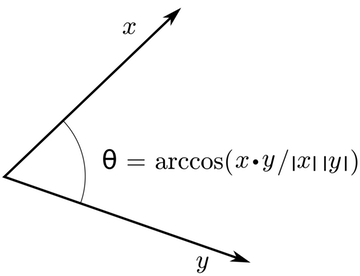
我们可以不计算实际的角度,而是把相似度保留为 $similarity = cos(\Theta)$ 的形式。形式上,两个向量 $p$ 和 $q$ 之间的 Cosine Similarity $s$ 定义为:
$$s = \frac{p \cdot q}{||p|| ||q||}, \textrm{ where } s \in [-1, 1] $$
cell 43
Question 2.2: Words with Multiple Meanings(多义词)(1.5 分)[code + written]
Polyseme(多义词)和 homonym(同形/同音异义词)是指具有不止一个含义的词(关于 polyseme 与 homonym 区别的更多内容,见这个 wiki page)。请找一个词,它要有至少两个不同的含义,且其 top-10 最相似词(按 cosine similarity)中同时包含来自两个含义的相关词。例如,"leaves" 的 top 10 里既有 "go_away" 的含义,也有 "a_structure_of_a_plant" 的含义;"scoop" 的 top 10 里既有 "handed_waffle_cone",也有 "lowdown"。你可能要试好几个多义词或同形异义词,才能找到一个。
请写出你找到的词,以及在 top 10 中出现的多个含义。你认为为什么你试过的许多多义词/同形异义词都不奏效(即 top-10 最相似词只包含该词其中一个含义)?
Note:你应当使用 wv_from_bin.most_similar(word) 函数来获得 top 10 最相似的词。该函数按照与给定词的 cosine similarity 对词表中的所有其他词进行排序。如需更多帮助,请查阅 GenSim documentation。
cell 44|代码(原件里的脚手架,原样保留)
# ------------------
# Write your implementation here.

# ------------------
cell 45
在此写下你的答案。
cell 46
Question 2.3: Synonyms & Antonyms(同义词与反义词)(2 分)[code + written]
在考虑 Cosine Similarity 时,通常更方便的是考虑 Cosine Distance,它就是 1 - Cosine Similarity。
请找三个词 $(w_1,w_2,w_3)$,其中 $w_1$ 与 $w_2$ 是同义词,$w_1$ 与 $w_3$ 是反义词,但 Cosine Distance $(w_1,w_3) <$ Cosine Distance $(w_1,w_2)$。
举例来说,$w_1$="happy" 与 $w_3$="sad" 的距离比与 $w_2$="cheerful" 更近。请另找一个满足上述条件的例子。找到例子后,请给出一个可能的解释,说明为什么会出现这种反直觉的结果。
你应当在这里使用 wv_from_bin.distance(w1, w2) 函数来计算两个词之间的 cosine distance。如需更多帮助,请参阅 GenSim documentation。
cell 47|代码(原件里的脚手架,原样保留)
# ------------------
# Write your implementation here.

# ------------------
cell 48
在此写下你的答案。
cell 49
Question 2.4: Analogies with Word Vectors(用词向量做类比)[written](1.5 分)
词向量已被证明有时能展现出求解类比的能力。
例如,对于类比 "man : grandfather :: woman : x"(读作:man 之于 grandfather,如同 woman 之于 x),x 是什么?
在下面的 cell 中,我们向你展示如何使用 GenSim documentation 中的 most_similar 函数,用词向量求出 x。该函数会找出与 positive 列表中的词最相似、且与 negative 列表中的词最不相似的词(同时会略去输入词本身,因为它们往往就是最相似的;见 this paper)。类比的答案将具有最高的 cosine similarity(即返回的数值最大)。
cell 50|代码(原件里的脚手架,原样保留)
# Run this cell to answer the analogy -- man : grandfather :: woman : x
pprint.pprint(wv_from_bin.most_similar(positive=['woman', 'grandfather'], negative=['man']))
cell 51
令 $m$、$g$、$w$、$x$ 分别表示 man、grandfather、woman 和答案的词向量。只使用向量 $m$、$g$、$w$ 以及向量算术运算符 $+$ 和 $-$,我们要最大化其与 $x$ 的 cosine similarity 的那个表达式是什么?
提示:回忆一下,词向量就是表示一个词的多维向量。用各向量任意摆放的位置画一个 2D 的例子,可能会有帮助。在坐标平面上,man 和 woman 相对于 grandfather 和答案会位于哪里?
cell 52
在此写下你的答案。
cell 53
Question 2.5: Finding Analogies(寻找类比)[code + written](1.5 分)
a. 对于上一个例子,显然 "grandmother" 才能补全这个类比。但请给出一个直观的解释,说明为什么 most_similar 函数会给出像 "granddaughter"、"daughter" 或 "mother" 这样的词?
cell 54
在此写下你的答案。
cell 55
b. 找一个按这些向量成立的类比例子(即目标词排在第一位)。在你的解答中,请按 x:y :: a:b 的形式写出完整的类比。如果你认为这个类比比较复杂,请用一两句话解释它为什么成立。
Note:你可能需要试很多个类比,才能找到一个可行的!
cell 56|代码(原件里的脚手架,原样保留)
# For example: x, y, a, b = ("", "", "", "")
# ------------------
# Write your implementation here.

# ------------------

# Test the solution
assert wv_from_bin.most_similar(positive=[a, y], negative=[x])[0][0] == b
cell 57
在此写下你的答案。
cell 58
Question 2.6: Incorrect Analogy(错误的类比)[code + written](1.5 分)
a. 下面,我们期望看到预期的类比 "hand : glove :: foot : sock",但实际看到的却是一个意外的结果。请给出一个可能的理由,解释为什么这个类比会得出这样的结果?
cell 59|代码(原件里的脚手架,原样保留)
pprint.pprint(wv_from_bin.most_similar(positive=['foot', 'glove'], negative=['hand']))
cell 60
在此写下你的答案。
cell 61
b. 再找一个按这些向量不成立的类比例子。在你的解答中,按 x:y :: a:b 的形式写出预期的类比,并根据词向量写出 b 的错误取值(在上一个例子中,这个值会是 '45,000-square')。
cell 62|代码(原件里的脚手架,原样保留)
# For example: x, y, a, b = ("", "", "", "")
# ------------------
# Write your implementation here.

# ------------------
pprint.pprint(wv_from_bin.most_similar(positive=[a, y], negative=[x]))
assert wv_from_bin.most_similar(positive=[a, y], negative=[x])[0][0] != b
cell 63
在此写下你的答案。
cell 64
Question 2.7: Guided Analysis of Bias in Word Vectors(词向量中偏见的引导性分析)[written](1 分)
意识到我们的 word embeddings 中隐含的偏见(性别、种族、性取向等)是很重要的。偏见可能很危险,因为使用这些模型的应用会借此强化刻板印象。
运行下面的 cell,考察 (a) 哪些词与 "man" 和 "profession" 最相似、且与 "woman" 最不相似,以及 (b) 哪些词与 "woman" 和 "profession" 最相似、且与 "man" 最不相似。指出女性关联词列表与男性关联词列表之间的差异,并解释它如何反映了性别偏见。
cell 65|代码(原件里的脚手架,原样保留)
# Run this cell
# Here `positive` indicates the list of words to be similar to and `negative` indicates the list of words to be
# most dissimilar from.

pprint.pprint(wv_from_bin.most_similar(positive=['man', 'profession'], negative=['woman']))
print()
pprint.pprint(wv_from_bin.most_similar(positive=['woman', 'profession'], negative=['man']))
cell 66
在此写下你的答案。
cell 67
Question 2.8: Independent Analysis of Bias in Word Vectors [code + written] (1 point)
使用 most_similar 函数,另找出一对能够说明这些向量体现出某种偏见的类比(analogy)。请简要解释你所发现的偏见示例。
cell 68|代码(原件里的脚手架,原样保留)
# ------------------
# Write your implementation here.

# ------------------
cell 69
在此写下你的答案。
cell 70
Question 2.9: Thinking About Bias [written] (2 points)
a. 给出一种可能的解释:偏见(bias)是如何进入 word vectors 的。你的解释应聚焦于 word vectors,而不是其他 AI 系统(例如 ChatGPT)中的偏见。如有必要,你可以用具体的历史事例来支撑你的解释。
cell 71
在此写下你的答案。
cell 72
b. 你可以用哪一种可能的方法来减轻 word vectors 所体现的偏见?请简要说明该方法,以及该方法的目标是什么。
cell 73
在此写下你的答案。
cell 74
Submission Instructions
- 点击 Jupyter Notebook 顶部的 Save 按钮。
- 选择 Edit -> Clear Outputs of All Cells。这会清除所有 cell 的输出(但会保留所有 cell 的内容)。
- 选择 Run -> Run All Cells。这会按顺序运行所有 cell,并需要几分钟时间。
- 重新运行完所有内容后,选择 File -> Save and Export Notebook as -> PDF(如果你看到类似 "nbconvert failed: Pandoc wasn't found" 的错误,可以先将它保存为 HTML)。选择 File -> Save and Export Notebook as -> HTML。这会把 notebook 保存为你电脑上的一个 HTML 文件。在网页浏览器中打开下载的 HTML 文件。在浏览器中按 Ctrl + P(Windows/Linux)或 Cmd + P(Mac)打开打印对话框。在打印对话框中,把目标(destination)改为 Save as PDF,然后点击 Save。 确保你所有的解答、尤其是编程部分都显示在 pdf 中,如果提供的代码因为代码 cell 中行不换行而被截断,那没关系。
- 查看 PDF 文件,确认你的所有解答都在、且显示正确。PDF 是评分者唯一会看到的东西!
- 在 Gradescope 上提交你的 PDF。
材料
官方地址(W26 ✓ 全部验证过可下载 ✓)。本地副本放
_local/(只服务本地、不外传)。
| 材料 | 链接 |
|---|---|
| 官方 notebook | a1.zip(0.1 MB) |
怎么自查
- 官方仓库自带的测试(
pytest/ sanity check)—— ⚠️ Gradescope 只对注册学生开放, 自学者以仓库自带测试为准; - 提交脚本:A3 / A4 提到
bash create_submission.sh。
这份作业和书的关系
见上表「配哪几讲」。等题面中英对照做完,这里会换成章节标题原文,并加定位校验
(指引指向一个不存在的标题会被 nav_check 报出来)。